Flávia F. Feitosa SER 301 – Análise Espacial de Dados Geográficos Introdução à Modelagem e Simulação Computacional.

Apresentação em tema: "Flávia F. Feitosa SER 301 – Análise Espacial de Dados Geográficos Introdução à Modelagem e Simulação Computacional."— Transcrição da apresentação:

1 Flávia F. Feitosa flavia@dpi.inpe.br SER 301 – Análise Espacial de Dados Geográficos Introdução à Modelagem e Simulação Computacional

2 Modelos Representações simplificadas de um objeto, estrutura, idéia ou sistema. São menores, menos detalhados, menos complexos, ou tudo isso junto… Podem ser estáticos ou dinâmicos… Y i =  0 + X i  1

3 Um mapa é um modelo? Representação simplificada de um estado do sistema de interesse. f Mas é estático! E os processos?

4 Modelos de Simulação (Computacional) Inclui a representação de determinados processos/comportamentos do sistema de interesse Propósito de compreender melhor o comportamento do sistema ao longo do tempo, dinâmicas não-lineares, retroalimentação do sistema…

5 Como comportamentos individuais geram padrões “macro” no nosso mundo... Um exemplo simples de simulação…

6 Bird Flocking o Nenhuma autoridade central o Cada pássaro reage ao seu vizinho o Modelo baseado em interações “bottom-up”

7 Bird Flocking Reynolds Model (1987) – Três regras www.red3d.com/cwr/boids/ Coesão: movimento em direção à posição média dos vizinhos/colegas. Separação: movimento buscando evitar aglomeração com outros colegas Alinhamento: manutenção da direção média dos vizinhos.

8 Bird Flocking Reynolds Model (1987) http://ccl.northwestern.edu/netlogo/models/Flocking

9 Complex Systems Systems composed of interconnected parts that as a whole exhibit one or more properties not obvious from the properties of the individual parts. Emergence Small number of rules applied locally among many individuals can generate complex global patterns Self-organization No centralized authority

10 Complex Systems Non-linearity Generate unexpected and counter-intuitive global patterns that cannot be understood as a simple sum of the parts. Invalidates simple extrapolation. Path-dependence Highly affected by past states Adaptation Adapt to unexpected changes in its environment (e.g. avoiding obstacles) Complicated vs. Complex

11 What are complex adaptive systems?

12 Traditional Modelling Approaches Statistical modeling, Classical optimization, System dynamics modeling… o Top-down view o Linear o Correlation o Cause and effect reasoning o Seeks to find some equilibrium representing the “solution” to the simulation o Often assume homogeneity o Some are static Simulation models  Are “run” rather than “solved”

13 Autômatos Celulares Liliam Medeiros

14 Agent-Based Modelling Another Alternative to traditional modeling paradigms What is an Agent? o Independent component (e.g. software object) representing a real world actor (family, government, …) o Have a state and behavioral rules o Behavioral rules determine moviments, interactions and changes in the agent’s state o The behavior can range from primitive reactive decision rules to complex adaptive intelligence. CRUCIAL o Capability to make independent decisions o Active rather than passive

15 Agent-Based Modelling Goal Environment Representations Communication Action Perception Communication Gilbert, 2003

16 Agents are… Identifiable and self-contained Goal-oriented –Does not simply act in response to the environment Situated –Living in an environment with which interacts with other agents Communicative/Socially aware –Communicates with other agents Autonomous –Exercises control over its own actions

17 Agents are… Reactive –Responds to changes in its environment Adaptive / Learning /Flexible –Changes its behavior based on its previous experience –Actions are not scripted Mobile –Able to transport themselves Temporally continuous –Continuously running process

18 Types of ABM Minimalist Models o Based on a set of idealized assumptions o Abstract and artificial o Exploratory laboratories in which assumptions can be tested o Ex: Schelling, Sugarscape Model Decision Support Models o Descriptive and realistic o Usually large-scale applications o Designed to answer real-world policy questions o Include real data to calibrate and to compare simulation outputs o Ex: MASUS (Multi-Agent Simulator for Urban Segregation) (Macal e North, 2005)

19 A Minimalist Model Schelling’s Model of Segregation Segregation is an outcome of individual choices But high levels of segregation mean that people are prejudiced?

20 Schelling’s Model of Segregation Schelling (1971) demonstrates a theory to explain the persistence of racial segregation in an environment of growing tolerance If individuals will tolerate racial diversity, but will not tolerate being in a minority in their locality, segregation will still be the equilibrium situation

21 Schelling’s Model of Segregation Schelling’s Model of Segregation < 1/3 Micro-level rules of the game Stay if at least a third of neighbors are “kin” Move to random location otherwise

22 Tolerance values above 30%: formation of ghettos http://ccl.northwestern.edu/netlogo/models/Segregation Schelling’s Model of Segregation

23 O Ciclo da Modelagem Definir o propósito do modelo, as questões que buscamos responder

24 O Ciclo da Modelagem Segregação é um resultado da intolerância das famílias em relação à presença de outros grupos sociais?

25 O Ciclo da Modelagem Formular hipóteses/premissas a partir de nosso conhecimento preliminar sobre como o sistema funciona

26 O Ciclo da Modelagem Se as famílias toleram a diversidade racial, mas não toleram ser a minoria em sua vizinhança, a situação de equilíbrio ainda apresentará altos níveis de segregação.

27 O Ciclo da Modelagem Quais elementos/interações a serem considerados? Como serão representados? Autômatos? Agentes? Escolher escalas, entidades, variáveis, processos e parâmetros do modelo

28 O Ciclo da Modelagem

29 Plataformas TerraME (INPE/UFOP) http://www.terrame.org NetLogo Northwestern's Center for Connected Learning and Computer-Based Modeling http://ccl.northwestern.edu/netlogo/ Repast (University of Chicago) http://repast.sourceforge.net/

30 O Ciclo da Modelagem Verificação, Comparação com Dados Reais, Simulação de Cenários, Análises de Sensibilidade

31 O Ciclo da Modelagem

32 Protocolo ODD (Overview, Design, Details) Grimm, V., Berger, U., Bastiansen, F., Eliassen, S., Ginot, V., Giske, J., John, G.-C., Grand, T., Heinz, S. K., Huse, G., Huth, A., Jepsen, J. U. & al., E. (2006) A standard protocol for describing individual-based and agent-based models. Ecological Modelling 198: 115-126. Grimm, V., Berger, U., DeAngelis, D. L., Polhill, J. G., Giske, J. & Railsback, S. F. (2010) The ODD protocol: a review and first update. Ecological Modelling 221: 2760-2768.

33 Overview Propósito o Que sistema estamos modelando? o O que estamos querendo aprender com isso? Entidades, Variáveis e Escalas o Tipos de entidades: um ou mais tipos de agentes, o ambiente onde agentes vivem e interagem (geralmente composto por unidades locais – células), ambiente “global”. o Variáveis que caracterizam cada uma dessas entidades (estáticas ou dinâmicas)

34 Overview Entidades, Variáveis e Escalas o Escala temporal: resolução e extensão temporal o Escala espacial: resolução espacial Process Overview and Schedule o Estrutura dinâmica do modelo o Quais os processos que modificam as variáveis que caracterizam as entidades do modelo? o Em que ordem estes processos ocorrem?

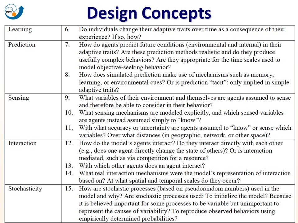
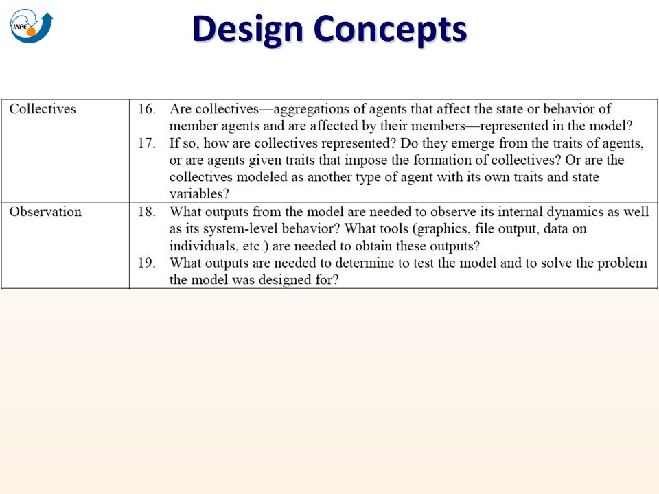
35 Design Concepts

36

37

38 Details Inicialização o Condições iniciais da simulação o Quantos agentes? Quais os valores iniciais das variáveis? Dados de Entrada o Arquivos de dados importados ao longo das simulações Sub-Modelos

39 Outros Exemplos de Modelos Minimalistas o Climate Change o Virus Transmission o Wealth distribution o …

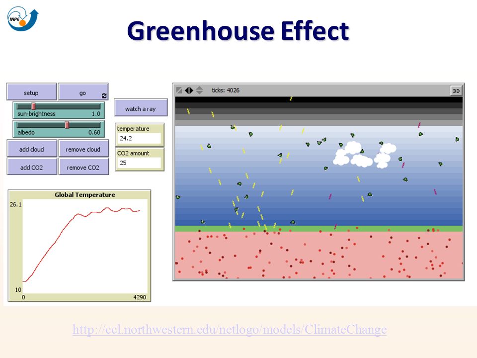
40 Greenhouse Effect

41 http://ccl.northwestern.edu/netlogo/models/ClimateChange

42 Greenhouse Effect BaselineAlbedoCO 2

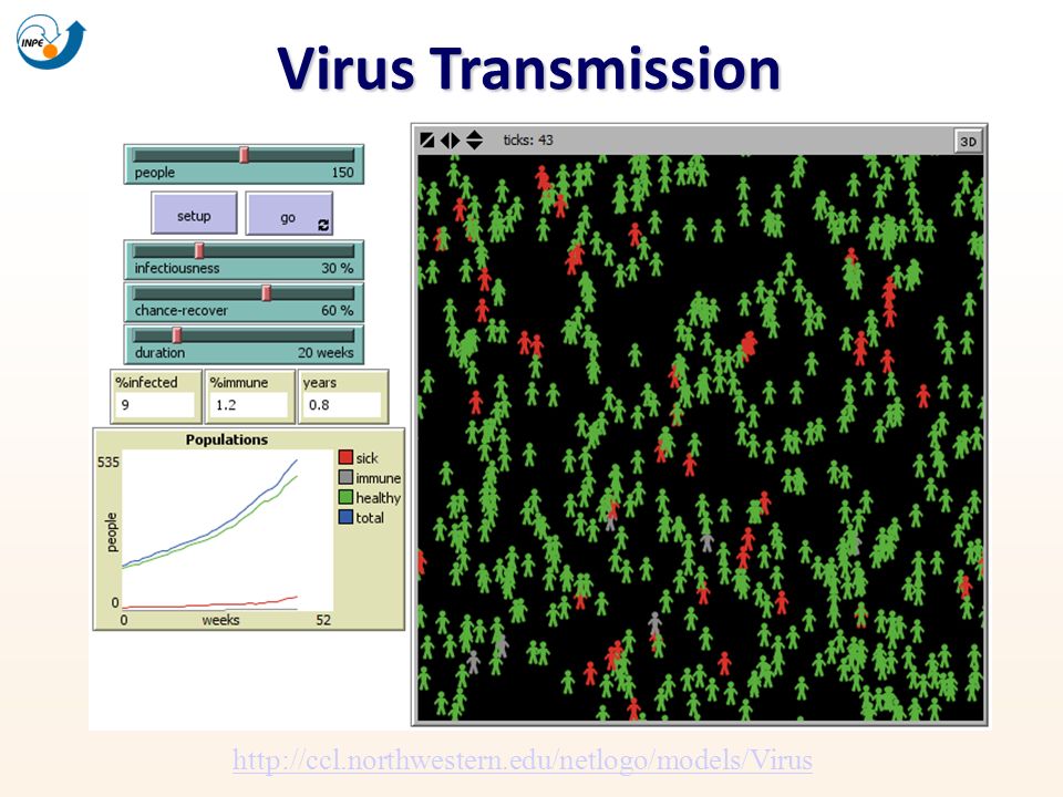
43 Virus Transmission

44 http://ccl.northwestern.edu/netlogo/models/Virus

45 Virus Transmission Baseline Recover >Recover <

46 Wealth Distribution Wealth Distribution Brazil ranks among the world's highest nations in the Gini coefficient index of inequality (G = 0.55) Source: Wikipedia

47 G = 0: Perfect equality (everybody has same wealth) G = 1: Perfect inequality (all is owned by one individual) Wealth Distribution: Gini Ratio Wealth Distribution: Gini Ratio

48 Wealth Distribution – Sugarscape Model Wealth Distribution – Sugarscape Model “The rich get richer and the poor get poorer” Sugarscape Model – Epstein & Axtell (1996) Illustrate Pareto’s Law Most of the people are poor, fewer are middle class, and very few are rich: 80/20 rule

49 Wealth Distribution – Sugarscape Model Agents o Collect grain and eat grain to survive o Grain accumulation = WEALTH o Vision: high is good o Metabolism: low is good Movement: move to cell within vision with more grains Replacement: Replace dead agent with random new agent Grain grows back with rate R

50 Wealth Distribution – Sugarscape Model Initial conditions: randomly distributed

51 Wealth Distribution – Sugarscape Model Uniform random assignments of vision and metabolism still result in unequal distribution of wealth HOW????

52 Wealth Distribution Non-linear distribution of wealth  Resembles a power law The "probability" or fraction of the population f(x) that owns a small amount of wealth per person (x) is rather high, and then decreases steadily as wealth increases PROBABILITY DENSITY FUNCTION Pareto Distribution

53 Decision Support Models

54 MASUS: Multi-Agent Simulator for Urban Segregation

55 Obstacles that contribute to perpetuate poverty Impacts of Segregation Policies to minimize segregation demand: A better understanding of the dynamics of segregation and its causal mechanisms

56 The Complex Nature of Segregation The Process Matters!

57 Multi-Agent Simulator for Urban Segregation MASUS Scientific tool to explore alternative scenarios of segregation Support planning actions by offering insights about the impact of policy strategiesPurpose Improve the understanding about segregation and its relation with different contextual mechanisms

58 MASUSMethodologicalSteps

59 MASUS Conceptual Model

60 MASUSMethodologicalSteps

61 São José dos Campos, Brazil São Paulo State Study Area City of São José dos Campos

62 MASUS: Process Schedule MASUS: Process Schedule

63 Decision-making sub-model ALTERNATIVES Not Move Move within the same neighborhood Move to the same type of neighborhood (n alternatives) Move to a different type of neighborhood (m alternatives) Higher probability to choose alternative with higher utility

64 Decision-making sub-model Decision-making sub-model Nesting Structure of the Model

65 NMNL: Affluent Households LevelChoiceVariableCoef.Std. err. 1 st Move Age of the household head-0.040 *** 0.011 Renter2.542 *** 0.425 Renter * household income-9.4(10 -5 )-7.5(10 -5 ) 2 nd Move within the same neigh.Constant-2.532 *** 0.693 Move to the same type of neighborhood Constant-2.464 *** 0.855 Type A neighborhood0.4770.661 Type B neighborhood0.0620.495 Kids * Type A-0.3680.636 Move to another type of neighborhood Constant-3.457 *** 1.053 Type A neighborhood-0.2560.732 Type B neighborhood1.760 *** 0.709 Kids * Type A1.49 ** 0.784 3 rd Generic variables Land price/ income-0.0840.053 Real estate offers1.4(10 -3 ) *** 5.1(10 -4 ) Distance from orig. neighborhood-4.9(10 -5 ) ** 2.5(10 -5 ) Distance to CBD2.3(10 -5 )2.9(10 -5 ) Prop. of high-income families0.960 ** 0.503

66 MASUS: Process Schedule MASUS: Process Schedule

67 MASUSMethodologicalSteps

68 Operational Model

69 MASUSMethodologicalSteps

70 Simulation Experiments Comparing simulation outputs with empirical data Testing theoretical issues Testing anti-segregation policy strategies

71 Comparison with Empirical Data Initial condition: São José dos Campos in 1991 Import GIS layers (households, environment) Import GIS layers (households, environment) Set parameters Set parameters Run 9 annual cycles Compare simulated results with real data (year 2000)

72 Comparison with Empirical Data Dissimilarity Index (local scale) Initial State (1991) Simulated Data (1991-2000) Real Data (2000) 0.54 0.31 0.15 0.51 0.30 0.19 0.51 0.30 0.19

73 Comparison with Empirical Data Isolation Poor Households (local scale) Initial State (1991) Real Data (2000) 0.54 0.51 Simulated Data (1991-2000)

74 Comparison with Empirical Data Isolation Affluent Households (local scale) Initial State (1991) Real Data (2000) 0.15 0.19 Simulated Data (1991-2000)

75 Testing a theory How does inequality affect segregation? Relation between both phenomena has caused controversy in scientific debates Experiment Compare 3 scenarios 1991-2000 Scenario 1: Previous run (baseline) Scenario 2: Decreasing inequality Scenario 3: Increasing inequality

76 Testing a theory Inequality (Gini) Proportion Poor HH Proportion Affluent HH Scenario 1 (Original) Scenario 2 (Low-Ineq.) Scenario 3 (High-Ineq.) Dissimilarity Isolation Poor HH Isolation Affluent HH

77 Testing policy strategies Experiment Compare 3 scenarios Scenario 1 no voucher (baseline) Scenario 2 200 – 1700 vouchers Scenario 3 400 – 4200 vouchers Poverty Dispersion vs. Wealth Dispersion Poverty Dispersion: housing vouchers to poor families

78 Testing policy strategies Scenario 1 No voucher (baseline) Scenario 2 200 - 1700 vouchers (2.3%) Scenario 3 400 - 4200 vouchers (5.8%) Dissimilarity Isolation Poor HH Isolation Affluent HH 2.3 - 3.5 % 5.8 - 10.7% 2.3 - 1.7 % 5.8 - 3.4% 2.3 - 5.7 % 5.8 - 8.3 %

79 Testing policy strategies Poverty Dispersion Demands high and continous investment to decrease poverty isolation Poverty Dispersion vs. Wealth Dispersion Slows down the increase in segregation, but does not change the trends

80 Testing policy strategies Poverty Dispersion vs. Wealth Dispersion Experiment Compare 2 scenarios Scenario 1 (baseline) Scenario 2 new areas for upper classes Urban areas in 1991 Undeveloped areas for upper classes Wealth Dispersion: Incentives for constructing residential developments for upper classes in poor regions of the city

81 Testing policy strategies Scenario 1 baseline Scenario 2 new areas for upper classes Dissimilarity Isolation Poor HH Isolation Affluent HH

82 Testing policy strategies Wealth Dispersion Produces long-term outcomes Poverty Dispersion vs. Wealth Dispersion More effective at decreasing large-scale segregation E.g. Dissimilarity 2010 local scale (700m): - 19% large scale (2000m): - 36%

83 Testing policy strategies Wealth Dispersion Positive changes in the spatial patterns of segregation Poverty Dispersion vs. Wealth Dispersion Baseline 2010 Wealth Dispersion 2010

84 Virtual laboratory for testing theories and policy approaches on segregation Does not focus on making exact predictions Exploratory tool, framework for assembling relevant information Multi-Agent Simulator for Urban Segregation MASUS

85 Um contador de histórias Modelos de simulação contam uma história A história pode ser boa ou não… Pode ser sobre o presente, passado ou futuro… FERRAMENTA PARA COMPARTILHAR VISÕES, LEVANTAR DÚVIDAS, ESTRUTURAR DISCUSSÕES E DEBATES Mas oferece uma outra maneira de examinar a situação!