Copolimerização Síntese e Modificação de Polímeros Aula 7 Prof. Sérgio Henrique Pezzin.

Apresentação em tema: "Copolimerização Síntese e Modificação de Polímeros Aula 7 Prof. Sérgio Henrique Pezzin."— Transcrição da apresentação:

1

2 Copolimerização Síntese e Modificação de Polímeros Aula 7 Prof. Sérgio Henrique Pezzin

3 Copolimerização é um tipo de polimerização a partir de uma mistura de dois (ou mais) monômeros para produzir copolímeros. A homopolimerização e os homopolímeros partem de apenas um tipo de monômero. Introdução

4 Importância da copolimerização Uma importante técnica de modificação de polímeros! Tem o objetivo de: (1) introduzir funcionalidades desejadas nos polímeros (2) avaliar a reatividade do monômero na polimerização e o mecanismo de polimerização

5 Exemplos Estireno + Butadieno SBR Acrilonitrila + Butadieno NBR Acrilonitrila + Butadieno + Estireno ABS Acrilato de Na + Álcool vinílico Resina de alta absorção de água

6 Dos exemplos, temos que 1. Usando técnicas de copolimerização, muitas propriedades podem ser muito melhoradas, tais como, resistência mecânica, elasticidade, plasticidade, Tg, solubilidade, tribologia, resistência química, anti-envelhecimento, etc. 2. Se necessário, um terceiro monômero pode ser empregado para melhorar as propriedades de materiais poliméricos.

7 Fatores importantes Para descrever a homopolimerização, usamos como fatores a velocidade de polimerização, a massa molecular e a distribuição de massa molecular. Diferente da homopolimerização, descrevemos a copolimerização usando fatores como a composição do copolímero e a distribuição de sequência.

8 Tipos de Copolímeros De acordo com as suas cadeias, os copolímeros podem ser classificados em quatro tipos: 1. Copolímeros aleatórios 2. Copolímeros alternados 3. Copolímeros em bloco 4. Copolímeros enxertados (graftizados)

9 Copolímeros Aleatórios Chamamos de poli(M 1 -co-M 2 ) tal como poli(butadieno-co-estireno) Unidade M 1 Unidade M 2

10 Copolímeros Alternados Os monômeros são ligados ordenadamente um a um Chamamos de poli(M 1 -alt-M 2 ) tal como poli(estireno-alt-anidrido maleico)

11 Copolímeros em Bloco existem diblocos,triblocos e multiblocos Tais como AB, ABA, ABC e (AB)n Bloco M 1 Bloco M 2 Chamamos poli(M 1 -b-M 2 ) ou copolímero em bloco(M 1 /M 2 ) tal como poli(estireno-b-butadieno) ou copolímero em bloco(estireno/butadieno)

12 Copolímeros Enxertados (Graft) backbone ramificação Chamamos de poli(backbone-g-branch) tal como poli(estireno-g-butadieno)

13 Em uma copolimerização típica, ocorrem alguns fenômenos interessantes, tais como: 1.uma diferença entre a razão dos monômeros em relação à composição do copolímero; 2.alguns pares de monômeros têm dificuldade de reagir entre eles, enquanto alguns monômeros podem reagir com outro monômero mas não reagem entre si mesmo. 3.Há uma discrepância de atividade entre diferentes tipos de monômeros. Composição de Copolímeros

14 Equação da Copolimerização Polimerização em Cadeia 1. Iniciação 2. Propagação 3. Terminação M 1 M 2: pares de monômeros ~~M 1 * ~~M 2 * : centros reativos

15 Iniciação da Cadeia K i1 K i2

16 Propagação da Cadeia

17 Terminação da Cadeia k 11 M 1 * + M 1 * Polímero R 11 =k t t [ M 1 * ] 2 t 12 k M 1 * + M * Polímero R =k t t [ M 1 * ] 2 t 2 [ M * ]

18 Aproximações para copolimerização Teoria da atividade igual: a reatividade do final da cadeia é independente do comprimento da cadeia. A reatividade de uma cadeia em crescimento depende apenas da unidade monomérica terminal. A maior parte dos monômeros é consumida durante a propagação.

19 Steady state da propagação:

20 Dedução da composição do copolímero

21 Considerações de steady state para M 1 * e M 2 *

22 definição

23 Equação da Copolimerização (Mayo-Lewis) Em que, 1. d[M 1 ]/d[M 2 ]: composição instantânea do polímero 2. [M 1 ]/[M 2 ] composição instantânea do monômero 3. r 1, r 2 razões de reatividade ~~M 1 * +M 1 k 11 r 1 =k 11 /k 12 ~~M 2 * +M 2 k 22

24 Outra forma da Equação de Mayo-Lewis Definição: f 1 = fração molar de M 1 no reator F 1 = fração molar de M 1 no copolímero

25 Discussão da Equação de Mayo-Lewis 1. Dá a composição instantânea do copolímero 2. Normalmente a composição do copolímero é diferente da razão entre os monômeros (feed ratio), exceto nos casos de r 1 =r 2 =1 ou r 1 [M 1 ]+[M 2 ]=[M 1 ]+r 2 [M 2 ]=1 3. Há diferentes tipos de centros ativos, tais como radicalares, aniônicos e catiônicos. r 1 e r 2 para cada par de monômeros será diferente para cada tipo de centro ativo 4. Para a copolimerização iônica, a razão de reatividade é muito afetada pelo contra-íon, solvente e temperatura.

26 Curva de Composição do Copolímero e tipo de copolymerização Razão de reatividade r é a razão entre as atividades do monômeros na propagação competitiva. r 1 =K 11 /K 12

27 A relação entre r 1 e o caráter da polimerização r 1 = 0 r 1 = 0 apenas copolimerização sem homopolimerização 0 < r 1 < 1 0 < r 1 < 1 o monômero tende à copolimerização e a copolimerização aumenta com o descréscimo de r; r 1 = 1 mesma tendência entre r 1 = 1 mesma tendência entre homo- and copolimerização 1 < r 1 <. 1 < r 1 < o monômero tende à homopolimerização e a homopolimerização aumenta com o aumento de r.

28

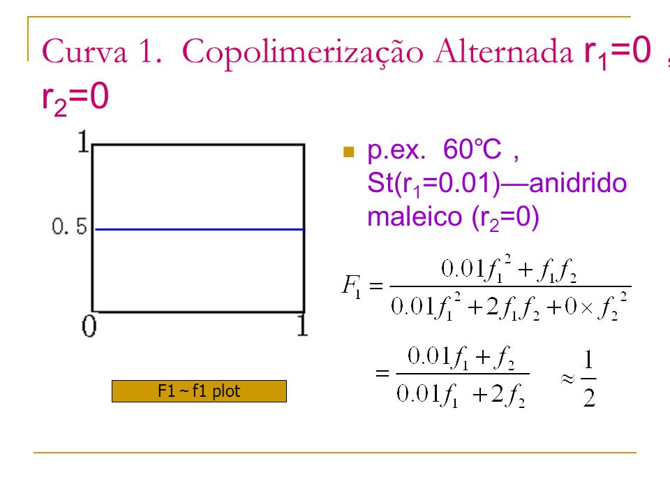
29 Curva 1. Copolimerização Alternada r 1 =0 r 2 =0 p.ex. 60 St(r 1 =0.01)anidrido maleico (r 2 =0) F1 f1 plot

30 Características 1) Apenas copolimerização, sem homopolimerização: k 11 =0, k 22 =0 2) Dois tipos de unidades monoméricas arranjadas alternadamente 3) Praticamente r 1 0 e r 2 0 ao invés de r 1 =r 2 =0. Quanto menor for r 1 *r 2, maior a tendência a uma copolimerização alternada.

31 Curva 2. r 1 <1 r 2 <1 com ponto azeotrópico r1=0.6 r2=0.3 R1=0.5 R2=0.5 F1 f1 plot A Ponto Azeotrópico

32 No ponto azeotrópico O azeótropo é importante, particularmente na indústria, porque neste ponto a composição monomérica e a do copolímero não mudam durante a conversão, produzindo, portanto, copolímeros homogêneos em composição. Copolimerizações sob outras condições irão alterar as composições instantâneas ao longo da curva de composição.

33 Curva 3. Copolimerização azeotrópica ideal r 1 =1 r 2 =1 F1 f1 plot

34 F 1 =f 1 e não mudam com o grau de conversão (copolimerização ideal) k 11 = k 12 k 22 = k 21 M 1 * e M 2 * têm a mesma reatividade com M 1 e M 2 p.ex. CF 2 =CF 2 CF 2 CFCl St p-MSt, 70

35 Curve 4. r 1 > 1 r 2 1 10 5 0.5 0.1 1) Se r 1 > 1 (k 11 > k 12 ) e r 2 < 1 (k 22 < k 21 ) M 1 é mais reativo que M 2 sem importar M 1 * e M 2 *. F 1 é sempre maior que f 1 e a curva está sempre acima da diagonal. A situação é similar for r 1 1 e, neste caso, a curva estará abaixo da diagonal.

36 2 S e r 1 x r 2 = 1 (r 2 =1/r 1 ), a copolimerização se torna ideal Neste caso M 1 * e M 2 * têm a mesma preferência para a adição de qualquer um dos dois monômeros.

37 Curva 5. r 1 >1 r 2 >1 Estireno(r 1 =1.38)/isopreno(r 2 =2.05)

38 Característica da Curva 5 1) Existe um ponto azeotrópico 2) Os pares de monômeros preferem homopolimerizar do que copolimerizar. Quando r 1 e r 2 >> 1, formam-se blocos ao longo da cadeia.

39 Equação Integrada para a Composição do Copolímero Importância do controle da composição nas propriedades do produto: SB rubber S 22 25 pneu S pneu rígido S resistência quando frio 1 A composição é projetada de acordo com as propriedades finais 2 A composição do copolímero varia com a conversão. Desafio: como preparar o copolímero com a composição desejada??

40 A influência da conversão na composição do copolímero a. Descrição Qualitativa p.ex. curva F1 f1 (r 1 <1,r 2 <1) No ponto A (azeótropo) (f 1 ) A =f 1 F 1 (f 1 ) A =f 1 ; No ponto B, (F 1 ) B decresce ao longo da curva com a conversão; No ponto C, o comportamento é contrário ao do ponto B.

41 F1 f1 curve (r 1 <1,r 2 <1) Conclusão a composição do copolímero muda com a conversão; os produtos são misturas de copolímeros com diferentes composições (distribuição de composição)

42 Equação Integrada Método de Skeist: Para um sistema binário, o número total de mols de pares de monômeros é M e F 1 >f 1 Quando dM de monômero é polimerizado, a unidade M 1 no copolímero aumenta em F 1 dM e a razão monomérica muda para f 1 -df 1.

43 Em que, Mf 1 o M 1 no sistema F 1 dM o M 1 no copolímero f 1 -df 1 após reagir dM de M 1 a razão de M 1 no sistema; (f 1 -df 1 )(M-dM) M 1 não reagido no sistema. Mf 1 (M-dM)(f 1 -df 1 ) = F 1 dM

44 dM.df 1 é desprezível e a equação pode ser escrita como Mdf 1 +f 1 dM=F 1 dM Daí temos que Equação de Skeist

45 Define o grau de conversão em mols

46 Meyer et. Al,

47 With certain value of r 1,r 2 and initial feed ratio f 0 1, we calculate the value of C,F 1,and f 1 The relation between average copolymer composition and conversion C,

48 Fração molar conversão 1 M/M 0 0.2 0.8 0 1.0 f1f1 F1F1 Média de M 1 no copolímero f2f2 F2F2 Média de M 2 no copolímero

49 5.2.4 Copolymer composition distribution and control methods 1 Copolymer composition distribution A. In figure 5 4 st r 1 =0.30 and diethyl fumarate r 2 = 0 07 azeotrope

50 f 1 =0.20 f 1 =0.40 f 1 =0.50 f 1 =0.80 f 1 =0.70 Azeotropic copolymer f 1 =0.57 Copolymerization of styrene and diethyl fumarate

51 Conclusion 1. If the monomer feed ratio is azeotrope, the composition does not change with conversion; 2. If the monomer feed ratio is close to azeotrope, the composition does not change greatly; 3. If the monomer feed ratio is far from azeotrope, the composition will change greatly and no well-proportioned copolymer.

52 (2) Copolymer composition control methods (1). one-pot method As r 1 1 r 2 1 and the copolymer composition of target copolymer is close to that of the azeotropic copolymer, then the monomer pairs can be fed at one pot according to the target ratio. e.g. As we want to prepare PSA with F1 0.55 St(r1=0.41)/AN(r2=0.04), we can adopt one-pot method because F 1 =0.62

53 (2) Adding the high reactivity monomer method Target to keep f1 approach to f1 0 method A. half-batch adding B. continuous adding

54 (a) (b) f10f10 f10f10 a)r1 f1,M1 consumed quick adding M1 b)R1 f1,M2 consumed quick adding M2

55 (c) f10f10 f10f10 F10F10 F10F10 c) r1>1,r2 f1) d) r1 1, normally adding M 2 (F1<f1) (d)

56 (3). Control conversion method If F 1 C curve has been got ahead (such as 5 4, r 1 =0.3, r 2 =0.07), the azeotrope (F 1 ) A =(f 1 ) A =0.57(horizontal line) 1) Curve 3 Since f 1 0 (=0.50) is close to (f 1 ) A F 1 slightly changed with C. Before C reach to 80 90 stop the reaction 2) Curve 4 f 1 0 =0.60 and the situation is similar to 3 3) Curve 1 Since f 1 0 (=0.20) is far from (f 1 ) A F 1 change greatly at small C. The reaction should be kept at low conversion 4) Curve 2 f 1 0 =0.80 and the situation is similar to 1. Normally we combined both method 2 and 3

57 1.In the typical copolymerization, there are some interesting phenomena, such as, 2.The difference between the monomer feed ratio to the product copolymer composition, 3.Some monomer pairs are difficult to react with each other, while some monomers can react with other monomer but not react with itself. 4.That is because of the discrepancy of activity between different kinds of monomers. Part 2 Copolymer Composition

58 5.2.1 Copolymer composition equation Chain polymerization 1. Initiation 2. Propagation 3. termination M 1 M 2: monomer pairs ~~M 1 * ~~M 2 * : reactive centers

59 Chain initiation K i1 K i2

60 Chain propagation

61 Chain termination k 11 M 1 * + M 1 * Polymer R 11 =k t t [ M 1 * ] 2 t 12 k M 1 * + M * Polymer R =k t t [ M 1 * ] 2 t 2 [ M * ]

62 Assumptions for copolymerization Activity equal theory: The reactivity of chain end is independent of chain length Reactivity of a growing chain depends only on the terminal monomer unit The most of monomers are consumed during the propagation and no depropagation

63 Steady state of propagation:

64 Deduction of copolymer composition

65 The steady state assumptions on M 1 * M 2 *

66 definition

67 Mayo-Lewis Equation In which, 1. d[M 1 ]/d[M 2 ]: instantaneous polymer composition 2. [M 1 ]/[M 2 ] instantaneous monomer composition 3. r 1 r 2 reactivity ratio ~~M 1 * +M 1 k 11 r 1 =k 11 /k 12 ~~M 2 * +M 2 k 22

68 Another form of Mayo-Lewis Equation (5 18) Definition:

69 Discussion of Mayo-Lewis Equation 1. Instantaneous copolymer composition 2. Normally copolymer composition is different from that of monomer pairs (feed ratio), except the case of r 1 =r 2 =1 or r 1 [M 1 ]+[M 2 ]=[M 1 ]+r 2 [M 2 ]=1 3. There are different kinds of active center, such as radical, anionic and cationic ion. The r 1 and r 2 of same monomer pairs should be different among different kinds of active center 4. For the ionic copolymerization, the reactivity ratio is greatly affected by the properties of anti-ion, solvent and temperature.

70 5.2.2 The copolymer composition curve and the type of copolymerization Reactivity ratio R is the ratio between the activity of monomer pairs in the competed propagation. r 1 =K 11 /K 12

71 The relation between r 1 and polymerization character r 1 = 0 only copolymerization but r 1 = 0 only copolymerization but no homopolymerization 0 < r 1 < 1 monomer tends to homopolymerization and the homopolymerization increase with the r decrease; 0 < r 1 < 1 monomer tends to homopolymerization and the homopolymerization increase with the r decrease; r 1 = 1 r 1 = 1 same ability between homo- and copolymerization 1 < r 1 < monomer tends to copolymerization and the copolymerization increase with the r increase;

72

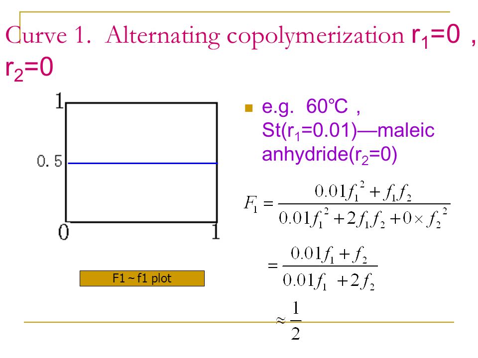
73 Curve 1. Alternating copolymerization r 1 =0 r 2 =0 e.g. 60 St(r 1 =0.01)maleic anhydride(r 2 =0) F1 f1 plot

74 character 1) Only copolymerization and no homopolymerization: k 11 =0, k 22 =0 2) Two kinds of monomer unit arrange alternatively F 1 F 2 take half of chains 3) Practically it is r 1 0 and r 2 0 instead of r 1 =r 2 =0. Smaller r 1 *r 2 is, stronger trends of alternative copolymerization shows.

75 Curve 2. r 1 <1 r 2 <1 with azeotrope point r1=0.6 r2=0.3 R1=0.5 R2=0.5 F1 f1 plot A Azeotrope point

76 At azeotrope point The azeotrope is important, particularly in industry, because the monomer and copolymer composition do not change with conversion, thus producing copolymers homogeneous in composition. Copolymerizations under the other conditions will change the instantaneous compositions along the composition curve.

77 Curve 3. Ideal azeotrope copolymerization r 1 =0 r 2 =0 F1 f1 plot

78 F 1 =f 1 and do not change with conversion (ideal copolymerization) k 11 = k 12 k 22 = k 21 M 1 * and M 2 * have same reactivity with M 1 and M 2 e.g. CF 2 =CF 2 CF 2 CFCl St p-MSt, 70

79 Curve 4. r 1 > 1 r 2 1 10 5 0.5 0.1 1) r1 > 1 (k11 > k12) and r2 < 1 (k22 < k21) shows that M 1 is more active than M 2 no matter for M 1 * and M 2 *. F 1 is always larger than f 1 and the curve is always above the diagonal. The situation is similar for r1 1 and the curve is below the diagonal.

80 2 as r1 * r2 = 1 (r 2 =1/r 1 ), it becomes ideal copolymerization In this case M 1 * and M 2 * have the same preference for adding one or the other of two monomers reactivity.

81 Curve 5. r 1 >1 r 2 >1 styrene(r 1 =1.38)/isoprene(r 2 =2.05)

82 Character of curve 5 The shape and position of curve 5 contrary to that of r 1 <1 r 2 <1; There is azeotrope point The monomer pairs prefer to homopolymerization rather than copolymerize. As r1 and r2 >> 1, the blocks form along the chain.

83 5.2.3 Integrated equation for copolymer composition The importance of composition control on product properties SB rubber S 22 25 tyre S stiff tyre S cold resistant 1 Composition is designed according to the final properties 2 The composition of products are normally different from that of materials; 3 The copolymer composition change with the conversion. Key: how to prepare the copolymer with the expected composition.

84 (1 The influence of conversion on the copolymer composition a. Qualitative description e.g. F1 f1 curve (r 1 <1,r 2 <1) At point A (azeotrope) (f 1 ) A =f 1 F 1 (f 1 ) A =f 1 ; At point B, (F 1 ) B decrease along the curve BO with conversion. At point C, it is contrary to that of point B.

85 F1 f1 curve (r 1 <1,r 2 <1) Conclusion the copolymer composition change with conversion; the products are mixtures of copolymers with different composition (composition distribution)

86 2. Integrated equation Skeist method: For a binary system, total molar number of monomer pairs is M and F 1 >f 1 As dM of monomer are polymerized, the M1 unit in the copolymer chain increase F 1 dM and the monomer ratio change to f 1 -df 1.

87 in which, Mf1 the M1 in the material F1dM the M1 unit in the copolymer f1-df1 after dM of M1 reacted the ratio of M1 in the material; (f1-df1)(M-dM) un reacted M1 in material. Mf 1 (M-dM)(f 1 -df 1 ) = F 1 dM ( 5-21 )

88 dM.df1 is neglected and then reset the above equation Mdf1+f1dM=F1dM We got Skeist Equation

89 Definite the mole conversion

90 ( 5-23a ) Meyer et. Al, ( 5-23b )

91 With certain value of r 1,r 2 and initial feed ratio f 0 1, we calculate the value of C,F 1,and f 1 The relation between average copolymer composition and conversion C, ( 5-24 )

92 0.2 0.8 Mole fraction conversion 1 M/M 0 0 1.0 f1f1 F1F1 average M 1 in copolymer f2f2 F2F2 average M 2 in copolymer

93 5.2.4 Copolymer composition distribution and control methods 1 Copolymer composition distribution A. In figure 5 4 st r 1 =0.30 and diethyl fumarate r 2 = 0 07 azeotrope

94 f 1 =0.20 f 1 =0.40 f 1 =0.50 f 1 =0.80 f 1 =0.70 Azeotropic copolymer f 1 =0.57 Copolymerization of styrene and diethyl fumarate

95 Conclusion 1. If the monomer feed ratio is azeotrope, the composition does not change with conversion; 2. If the monomer feed ratio is close to azeotrope, the composition does not change greatly; 3. If the monomer feed ratio is far from azeotrope, the composition will change greatly and no well-proportioned copolymer.

96 (2) Copolymer composition control methods (1). one-pot method As r 1 1 r 2 1 and the copolymer composition of target copolymer is close to that of the azeotropic copolymer, then the monomer pairs can be fed at one pot according to the target ratio. e.g. As we want to prepare PSA with F1 0.55 St(r1=0.41)/AN(r2=0.04), we can adopt one-pot method because F 1 =0.62

97 (2) Adding the high reactivity monomer method Target to keep f1 approach to f1 0 method A. half-batch adding B. continuous adding

98 (a) (b) f10f10 f10f10 a)r1 f1,M1 consumed quick adding M1 b)R1 f1,M2 consumed quick adding M2

99 (c) f10f10 f10f10 F10F10 F10F10 c) r1>1,r2 f1) d) r1 1, normally adding M 2 (F1<f1) (d)

100 (3). Control conversion method If F 1 C curve has been got ahead (such as 5 4, r 1 =0.3, r 2 =0.07), the azeotrope (F 1 ) A =(f 1 ) A =0.57(horizontal line) 1) Curve 3 Since f 1 0 (=0.50) is close to (f 1 ) A F 1 slightly changed with C. Before C reach to 80 90 stop the reaction 2) Curve 4 f 1 0 =0.60 and the situation is similar to 3 3) Curve 1 Since f 1 0 (=0.20) is far from (f 1 ) A F 1 change greatly at small C. The reaction should be kept at low conversion 4) Curve 2 f 1 0 =0.80 and the situation is similar to 1. Normally we combined both method 2 and 3

101 The copolymers with same composition often have different microstructure. A.alternating copolymer B.bi-block copolymer C.random copolymer (normal case) D.graft copolymer Part 3 Microstructure and Sequence Distribution

102 Segment length distribution function and average segment length By using probability method, the ratio of different length of (M l ) x and (M 2 ) y segments in macro-chain can be calculate, which is named as Segment length distribution.

103 Segment length distribution 1M 1 2M 1 4M 1 2M 1 3M 1 M 2 M 1 M 2 M 1 M 1 M 2 M 1 M 1 M 1 M 1 M 2 M 2 M 1 M 1 M 2 M 1 M 1 M 1 M 2 Competent reaction

104 Reaction probability P 11 and P 12 is P 11 +P 12 =1

105 similarly P 22 +P 21 =1

106 The probability which forms xM 1 segment from M 2 M 1 · to join with x-1 of M 1 unit and then with M 2 unit Segment sequence number distribution function similarly

107 Segment length sequence weight distribution function:the ratio of monomer unit in the chains to the total monomer

108 similarly

109 The number average length of xM 1 segment Total chain length Total chain nubmbers

110 similarly

111 Discusion on figure 5 6 and table 5 3 condition r1=5,r2=0.2, M1/M2=1 The probability of different length of M1 sequence: 1M 1 : PM 1 ) 1 =(5/6) 0 (1/6)=16.7% 2M 1 : PM 1 ) 2 =(5/6) 1 (1/6)=13.9% 3M 1 : PM 1 ) 3 =(5/6) 2 (1/6)=11.5% ……………… Ref to table 5 3 and figure 5 6a.

112 Length of M 1 unit, N M1 Probability of xM 1 segment (P M1 ) x,% The number of M 1 in xM 1 segment x(P M1 ) x,% 116.7 2.78 213.927.84.63 311.534.53.75 49.639.46.06 58.040.06.67 6 40.06.67 75.5538.96.49 84.6337.06.17 93.8533.85.64 103.2132.15.35 200.5210.41.74 300.0842.520.42 400.01360.540.09 500.00220.110.018 ………… (P M1 ) x =100 % x(P M1 ) x =60 0%=6 100%

113 Figure 5-5 segment distribution(a) and unit distribution(b) in copolymer a b

114 From figure 5 6a, we can get, 1. the shape of figure is similar to molecular weight number distribution curve 2. the meaning the percentage of xM1 segment in ΣxM1 16.7% of 1M1…13.9% of 2M1… 8.0% of 5M1……… 3. the ratio of 1M1segment is the highest, which can be refed to the highest ratio of x=1 monomer in the molecular weight number distribution curve

115 According to the probability theory,the copolymer composition ratio d[M 1 ]/d[M 2 ] is the nubmer-averaged length ratio between two segments.

116 Part 4 The Rate Equation of copolymerization Initiation, propagation and termination The effect of termination rate on copolymerization rate 1. The chemical controlled termination; 2. The diffusion controlled termination.

117 5.4.1 The rate equation of chemical controlled termination Since the dispear rate of monomer is determined by propagation, the overall propagation rate is the sum of four kinds of propagation.

118 Two kinds of steady asumption 1. The concentration of all kinds of radicals are in the steady state then 2. The total concentration of radicals keep constant, I.e. the initiation rate equals to the termination rate R i = R t = 2k t11 [M 1 · ] 2 +2k t12 [M 1 · ][M 2 · ]+2k t22 [M 2 · ] 2

119 φ 1 is prefer to the cross termination

120 5.4.2 The rate equation of diffusion controlled termination The termination rate is depends on the viscosity of system as the viscosity is low. In the other word the chain termination is controlled by chain diffusion from the low conversion on. Therefore, the totoal propagation rate equation is

121 ( 5-36 )

122 The termination rate constant can be regarded as the function of termination rate constant of homopolymerization as fellows,

123 Eq.(6-29) Eq.(6-30) Figure 5-7 VAc-MMAsolvent copolymerization(60 )

124 Part 5 Experimental Evaluation of reactivity ratio It is key to recognize copolymer composition, microstructural sequence distribution, copolymerization rate, the related activity of monomer pairs Determination methods From the determination of copolymer composition, sequence distribution and copolymerization constant to the evaluation of reactivity ratio.

125 5.5.1 Determination methods of reactivity ratio 1 From the determination of copolymer composition A. At low conversion usually <5 or 10 B. By using the differential equation 5-15 or (5-18) 5 18

126 At higher conversion the integral equation (5-23b) is used instead of above equation: 5 23b

127 Techniques for copolymer analysis: elemental analysis infrared spectroscopy NMR Gas chromatography

128 From the determination of segment length distribution of (PM 1 ) x and (PM 2 ) x to calculate the reactivity ratio

129 Essential To analysis the microstructure difference of biads or triads and tetrads M 2 M 1 M 2 M 1 M 1 M 2 M 2 M 1 M 2 M 1 M 1 M 1 M 2 M 1 M 2 M 2 M 2 M 1 M 1 M 2 6 kind s of triad s 3 kinds of biads 9 kinds of tetrad s

130 e.g. The content of M 1 M 1 M 1,M 1 M 1 M 2,M 2 M 1 M 2 can be determined by NMR, which are named as A 111, A 112 and A 212, respectively. By using the following equation, (PM 1 ) 3 =A 111 /(A 111 +A 112 +A 212 ) (PM 1 ) 2 =A 112 /(A 111 +A 112 +A 212 ) (PM 1 ) 1 =A 212 /(A 111 +A 112 +A 212 ) the P 11 and r 1 can be calculated according to eq.(6-22) and (6-18). Similarly, P 22 and r 2 are obtained. The peaks corresponding to the different triads can be observed by NMR

131 termination is controlled by diffusion rate

132 by using steady-state assumption: (6-31) K p,k 11 and k 22 can be Determined by nonsteady- State polymerization Non-steady-state polymerization pulsant laser technique

133 5.5.2 Reactivity calculation method To determine the copolymer composition at low conversion 1 curve fitting method 2 line intersection method 3 Fineman-Ross method ( )

134 1 curve fitting method draw f1-F1 curve a series of experimental f1/F1 Compared with the curve draw by the preset reactivities r1 r2

135 f1f1 F1F1

136 2 line intersection reset 5-15 5 39 The lines with the variable value of r 1 and r 2 Ref to figure 5-8

137 Figure 5-8 the reactivity by line intersection method, in which the circular stand the most reasonable r 1 and r 2

138 By using the integral copolymer composition equation 5 40

139 3 Fineman-Ross method ( ) set x =[M 1 ]/[M 2 ] y =d[M 1 ]/d[M 2 ] eq. 5-39 is turned into 5 41a 5 41b

140 Figure 5-9 the reactivity of allyl chloride (M 1 ) and VAc (M 2 ) by FR equation treat with eq.(5-41b) treat with eq.(5-41a)

141 Yezrielev

142 5.5.3 The influence factors of reactivity r=k 11 /k 12, the factors which influence the k are also influence r Extra factors reaction condition Temperature Pressure solvent Intra factor structure factors

143 1 temperature reactivity ratio: r 1 k 11 /k 22 (5-42) Active energy of self-propagation Active energy of cross-propagation The small data shows that the reactivity ratio is not greatly influenced by reactivity ratio

144 A. R is not greatly influenced by T E is as little as c.a. 20 35kJ/mol,E 11 -E 12 is even little B. r1 with T increases and tends to ideal copolymerization that is, r1 < 1 T r 1 r1 > 1 T r 1 explanation if r 1 E 12, With T, k 11 >k 12, then k 11 /k 12 Therefore T r 1 1 Think of the case r 1 > 1

145 Table 5-4 the influence of temperature on reactivity ratio

146 2 Pressure Similar to the influence of temperature on reactivity ratio, the copolymerization tends to ideal copolymerization with pressure increases. e.g. For the copolymerization of MMA and AN at 1, 100, 1000 atm., the corresponding r 1 ·r 2 value is 0.16 0.54 and 0.91 respectively.

147 3 the polarity of solvent Radical copolymerization slightly influence on r (table 5-5) Ionic copolymerization greatly influence on propagation rate and r, because the polarity of solvent influence the properties of ion pairs, the forms and the ratio of active centers. Table 5-5 the reactivity ratio of styrene(M 1 )-methyl methacrylate(M 2 ) in different solvent

148 (4 other factors The pH of media MAA / DMAEMA The salt of Lewis acid In the presence of ZnCl 2, the copolymerization of St and MMA tends to the ideal copolymerization. Polymerization method the copolymerization of styrene and methene oxalic acid.

149 Part 6 the activity of monomer and Q,e scheme 1. The experimental methods for checking the activity of monomers and radicals 2. The influence of structural factors,such as resonance effects and steric effects, on the activity of monomers and radicals 3. Q,e scheme is the bridge between the activity of monomers and radicals and can be estimated the reactivity ratio of monomer pairs.

150 we can not distinguish the activity of monomers and radicals in the homopolymerization.

151 Why ? 1) Kp of propagation is not only depends on M, but also M * ; 2) there are lack of the frame of reference.

152 5.6.1 the relative activity of monomers Reciprocal of reactivity ratio 1 r 1 = k 12 k 11 It stand for the ratio of the propagation constant of a radical with another monomer to that with its mother monomer We can use 1/r 1 to compare the relative activity with a series of M2

153 The copolymerization of M 1 * with different second monomer

154 Table 5-6 the relative activity of vinyl monomer to various chain radicals (1/r 1 ) B S MMA methyl vinyl ketone AN MA VDC VC VAc VAc * - 100 67 20 10 4.4 1.0 MMA * 4 2.2 1.0 - 0.82 0.52 0.39 0.10 0.05 S * 1.7 1.0 1.9 3.4 2.5 1.4 0.54 0.059 0.019

155 The data in the table show the activity of the monomers towards the same radical The activity of monomers in the table decrease from the top to the end e.g. VAc * For the conjugation system with the radicals S * and B *, the activity of some monomers is deregulation.

156 Conclusion The activity of monomers with different substitute groups are in the following order CH 2 =CHX: C 6 H 5 -, CH 2 =CH- > -CN, -COR > - COOH, -COOR > -Cl > -OCOR, -R > -OR, -H The relative activity of CH 2 =CHX shows the influence of X on the activity of monomers a)the monomers with conjugation substitute group, such as B, S, have the biggest activity. b)the monomers with strong electron-attracted substitute group, such as AN, MMA, also have good activity. c) the monomers with electron-repulsion substitute group, such as VAc CH 2 =CHOR, has smallest activity.

157 5.6.2 the relative activity of radicals from r 1 = k 11 k 12 and the available k P r1, we can calculate k 12 = k 11 /r 1 = (k P /r 1 ) see table 5-7 K 12, k 1 2,k 1 2,show the relative activity of series of radicals towards same monomer M 2

158 Table 5-7 k 12 of the reaction of chain radical and monomer (L·mol -1 ·s -1 ) B S MMA AN MA VAc VC S 40 145 1550 49000 14000 230000 615000 MA 130 203 367 1310 2090 23000 209000

159 the data of rows in table 5-7show the relative activity of series of radicals towards same monomer E.g. the first row shows the activity of series radicals towards monomer B The activity of radicals increase from left to right The relation between table 5 6(1/r1) and table 5 7(k 12 =k 11 /r1) The columns in table 5 7 show the activity of series monomer towards the same radical

160 Conclusion 1.the activity of monomers are reverse to that of radicals 2.the influence of substitute groups on the activity of monomers and radicals are in different extent the influence of radicals > that of monomer

161 5.6.3 The structural factors which influence the activity of monomers the influence of substitute group of double bond on the activity of monomer and radical (1) conjugate effect (2) polarity effect (3) steric hindrance effect

162 (1 conjugate effect The influence of substitute group on monomers is reverse to that of radicals due to the conjugate effect If X is C 6 H 5 CH 2 CH 2 it can form p-π conjugate structural electron pair with radicals. The stability of system The activity of monomer is large and that of radical is small

163 e.g. the activity of styrene and butadiene radical is low, While their radicals are high If the conjugate effects of OCOCH 3 group of Vac is weak the activity of Vac is low and that of VAc.* is high.

164 Potential energy New radical 1. M * +M=D 2. M * +M s =D Morse curve distance Activation energy Reaction heat Activation energy 1>2, Rate 1<2

165 From above figure

166 Summary 1. The homopolymerization rate of monomers with conjugate substitute group are quicker than that of monomers without substitute group VAc ( k p =2300 ) > St (k p =145 ) 2.If both M1 and M2 have conjugate substitute group (or have not conjugate substitute group), the copolymerization is easy. (the monomers have similar activity)

167 3. If only one of monomer has substitute group and another monomer has not, the copolymerization is difficult. e.g. VAc St [smack of St plays the role of inhabitant agent on the polymerization of Vac]

168 2 Polar Effect There are some special cases, such as that of AN 1) For the radicals such as MMA *,MA *,VAc *, the activity is normal. AN < butadiene St, MMA 2) For the radicals such as S *,B *, the activity of AN are higher than the normal case AN > S B MMA

169 The polar effect is also know as the alternation effect the electron-pushing substituents slightly increase the density of the electron cloud (electronegative ), while the electron-pulling substituents slightly decrease the density of the electron cloud (electropositive ). These two types of monomer prefer to the alternative copolymerization.

170 Table 5-8 1) The tendency towards the alternative copolymerization is increased with the increase of the distance of monomers and the polarity of monomers. [r 1 r 2 0] 2) the monomers which is difficult to be homopolymerized can be copolymerized with the monomers whose polarity are exact opposite. maleic anhydride, diethyl fumarate St CH 2 =CHOR maleic anhydride trans-2-styrene

171 explanation 1. Free radical mechanism 1) Alfrey, Price : static effect between the electron donor (monomer) and electron acceptor leads to the decrease of activation energy. Therefore, the reaction become easy 2) Walling, Mayo The lowering of the energy of the transition state occurs by the electron transfer between radicals and monomers. 2. Complexes mechanism 1946 Bartlett, Najaki

172 3 Steric effect Depends on the bulk, location and numbers of substituents 1) 1,1-bisubstituent (at same carbon atom) small steric effects The two substituents are located at different atoms Obvious steric effects Activity of monomer increase Activity of monomer decrease

173 example CH 2 =CHCl k 12 =10000(react with VAc * ) CH 2 =CCl 2 k 12 =23000(react with VAc * ) the steric effects are obvious for the 1 2 substituent cis-1,2 dichloroethylene k 12 =370(react with VAc * ) trans-1,2 dichloroethylene k 12 =230(react with VAc * ) 2) 3 4 substituent

174 5.6.3 the structural factors influence on the activity of monomers Table 5-9 the reaction rate constant k 12 of monomer and radical

175 5.6.4 Q,e scheme A quantitative equation is set up by integrating the reactivity ratio, conjugate effect, polar effect and steric effect, in order to describe the relation of structure and performance.

176 Q-e Scheme was suggested by Alfrey- Price in 1974 to combine the rate constant of radicals and monomers with the conjugate effect and polar effect. P 1, e 1 Q 1, e 1 P 1, e 1 Q 2, e 2 K 12 = P 1 Q 2 exp(-e 1 e 2 )

177 In which, P 1 P 2 the activity of radical M 1 *, M 2 * Q 1 Q 2 the activity of M1 M2 e 1 e 2 the polarity of M1, M1 *, and the polarity of M2, M2 *, assuming the polarity of monomer equals to that of the corresponding radical

178 k 11 k 22 and k 21 can be expressed as 5 44 5 45 ln(r 1 r 2 )=-(e 1 -e 2 ) 2 5 46

179 Set Q = 1.0 e=-0.8 of styrene as criterion, Q,e of other monomers are given in the table 5 10

180 Table 5-10 Q.e data of monomers

181 Significance of Q,e Q shows the conjugate effect of monomer. A large Q stand for the high active of M and the low active of radical: Bd Q=2.39 > St Q=1.0 > VAc( Q=0.026) E shows the polar effect of monomer and radical. AN e 1.20 > VAc e=-0.22 Q-e scheme

182 Q e scheme figure 5-10 if the abscissa data of one monomer is far from that of another,the difference of the relative activity between monomers is large. In the other words, the copolymerization is difficult. if the ordinate data of one monomer is far from that of another,the difference of the polar effect between monomers is large. The reaction tends to alternative copolymerization. If both Q and e of two monomer is similar, the reaction tends to ideal copolymerization.

183 Part 7 Ionic Copolymerization The copolymer composition equation is also well used in the cationic, anionic and catalyst copolymerization. Since the activity center is different, the reactivity ratio of monomer pair is different in different copolymerization.Therefore, the ionic copolymerization show the different feature to the radical copolymerization.

184 1. High selectivity of monomers Radical copolymerization The monomer pair with the close data of Q,e tends to the ideal copolymerization. The monomer pair with the large difference of e tends to alternative copolymerization. Ionic copolymerization The electron-pushing monomer can be carried out with cationic copolymerization. The electron-pulling monomer can be carried out with anionic copolymerization. The electron-pushing monomer can not be copolymerized with the electron-pulling monomer.

185 example copolymerization of St(Q 2 =1.00 e 2 =-0.80) and MMA(Q 2 =0.74 e 2 =0.40). IType T( ) r1r2 AIBNR.R. 600.520.46 SnCl 4 R+R+ 2010.50.1 NaR-R- -300.126.4

186 Figure 5-11 styrene(M 1 )-MMA(M 2 )copolymer composition curve (feed ratio 1:1) radical anionic cationic

187 2. The ionic copolymerization tends to ideal copolymerization ln(r 1 -r 2 )=-(e 1 -e 2 ) 2 the similar polarity e 1 e 2, ln(r 1 r 2 ) 0 i.e., r 1 r 2 1

188 3. The effect of condition on reactivity ratio is obvious and complicated Solvent and temperature Radical copolymerization:slightly influence Ionic copolymerization obvious influence due to the influence on the decomposition of active center Anti-ion The obvious influence of the structure of initiator

189 By using the above factors, the copolymer composition can be adjustified. example: The reactivity ratio of monomers in cationic copolymerization are obviously affected by the polarity and solubility of solvent. The effects are enhanced with increasing the polarity difference of monomer pairs.

190 Table 5-11 the effects of solvent on reactivity ratio (AlBr 3,0 )

191 The influence of temperature on reactivity ratio of ionic copolymerization is bigger than that of radical copolymerization. example For the cationic copolymerization of isobutene and styrene, r 1 increase to 15 times from -90 to -30 and r 2 increase to 3 times.For the radical copolymerization of methyl styrene and p-chloroted styrene, r 1 decrease from 28 to 15 and r 2 increase from 0.12 to 0.28 from -78 to0.

192 The features of ionic copolymerization is similar to the ionic homopolymerization Firstly, the influence of monomer structure on activity is obvious. example the activity order of monomers in anionic copolymerization styrene p-methyl styrene p-methoxy styrene trimethyl styrene Additionally, the monomer with high activity in homopolymerization has also high activity in copolymerization (table 5-12).

193 Table 5-12 Rate constants and reactivity ratio of some monomers (in THF,25,anti-ion is Na + )

194 Secondly, there are great influence of reaction condition on activity. The influence of reaction condition of temperature, solvent and initiator type, on the reactivity ratio is much obvious in the ionic copolymerization than that in the radical copolymerization.