Um pouco mais sobre modelos de objetos. Ray Path Categorization Ray Path Categorization. Nehab, D.; Gattass, M. Proceedings of SIBGRAPI 2000, Brazil,

Apresentação em tema: "Um pouco mais sobre modelos de objetos. Ray Path Categorization Ray Path Categorization. Nehab, D.; Gattass, M. Proceedings of SIBGRAPI 2000, Brazil,"— Transcrição da apresentação:

1 Um pouco mais sobre modelos de objetos

2 Ray Path Categorization Ray Path Categorization. Nehab, D.; Gattass, M. Proceedings of SIBGRAPI 2000, Brazil, 2000, pp. 227-234.

3 Ray Path Categorization -

4 Curvas e Superfícies modelagem paramétrica

5 Requisitos: Independência de eixos x y x' y'

6 Requisitos: Valores Múltiplos x y

7 Requisitos: Controle Local x y

8 Requisitos: Redução da Variação polinômio de grau elevado

9 Requisitos: Continuidade Variável

10 Requisitos: Versatilidade

11 Requisitos: Amostragem Uniforme s 1 s 2 s 3 s 4 s n s i s j Formulação matemática tratável Finalizando:

12 Solução Curva representada por partes através de polinômios de grau baixo (geralmente 3) t=0 t=1 Parametrização t=0 t=1t=0 t=1 t=0 t=1 u0u0 u1u1 u2u2 unun

13 Curvas de Bézier P. de Casteljau, 1959 (Citroën) P. de Bézier, 1962 (Renault) - UNISURF Forest 1970: Polinômios de Bernstein x P(t) y z t=0 t=1 V0V0 V1V1 V2V2 V3V3 V n-1 VnVn onde: coef. binomial pol. Bernstein

14 Bézier Cúbicas x P(t) y z V0V0 V1V1 V2V2 V3V3

15 Polinômios Cúbicos de Bernstein 1 1 0 t B 0,3 (1-t) 3 3 1 0 t B 1,3 3(1-t) 2 t 1 1 0 t B 3,3 t3t3 1 0 t B 2,3 3(1-t) t 2 -3 1 1 0 t B 0,3 + B 1,3 + B 2,3 + B 3,3

16 Propriedades da Bézier Cúbica x P(t) y z V0V0 V1V1 V2V2 V3V3 R(0) R(1)

17 Controle da Bézier Cúbica

18 Redução de n=3 para n=2 Bezier n=2

19 Redução de n=2 para n=1 Bezier n=1

20 Cálculo de um Ponto (1-t) t Mostre que:

21 Subdivisão de Bézier Cúbicas...

22 Construção de uma Bezier u=1/2 P(1/2)

23 Introduction to Subdivision Surfaces Adi Levin

24 Subdivision Curves and Surfaces Subdivision curves –The basic concepts of subdivision. Subdivision surfaces –Important known methods. –Discussion: subdivision vs. parametric surfaces.

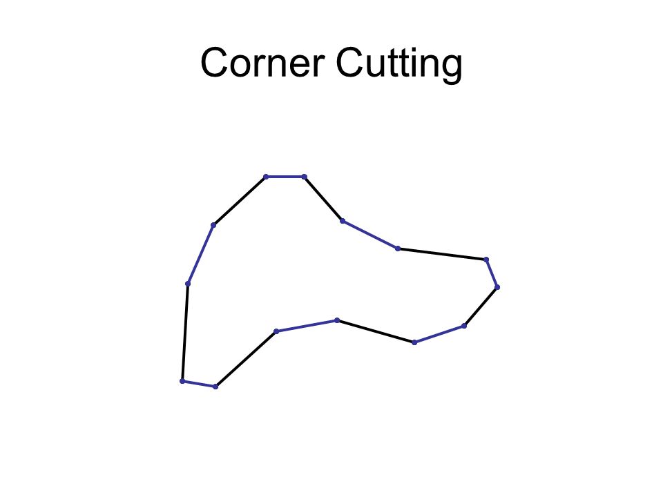
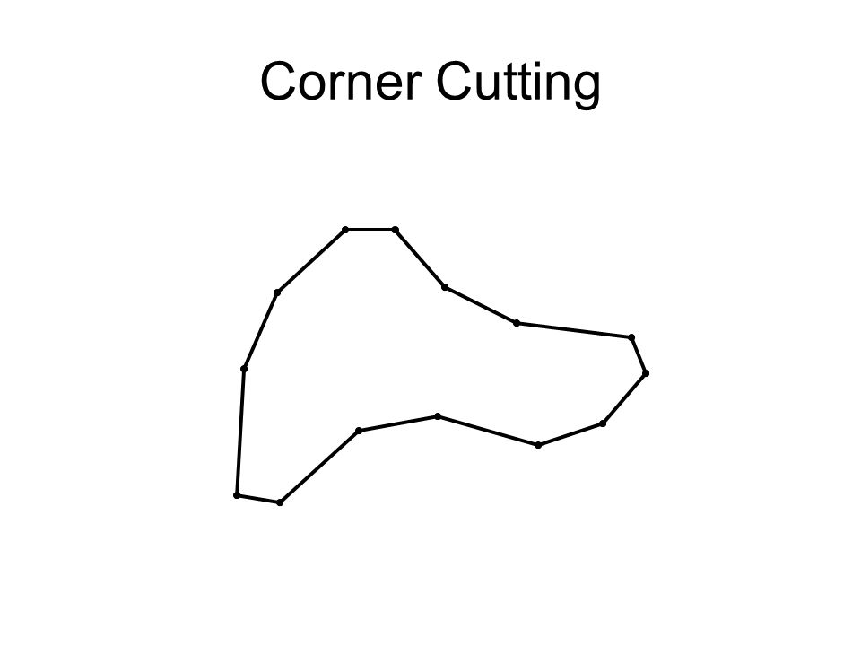
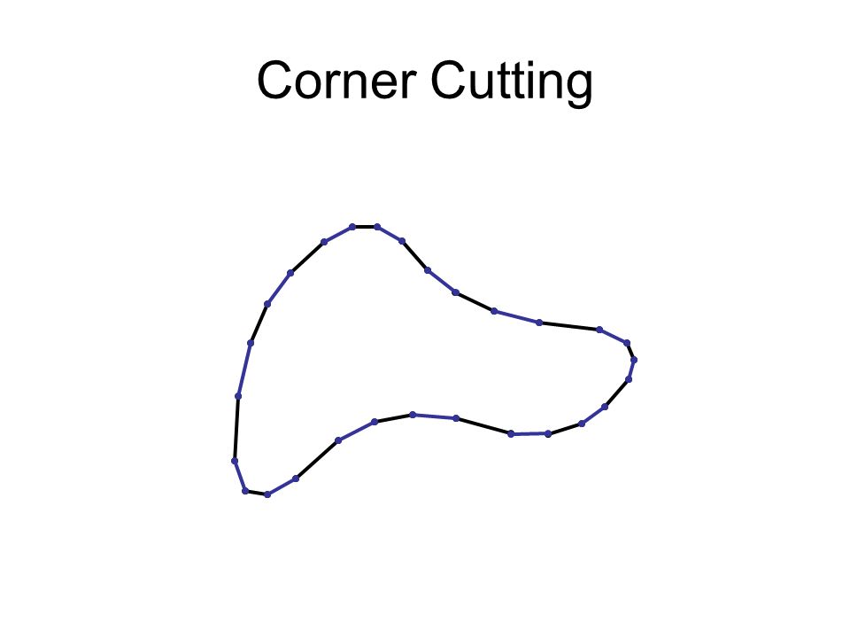
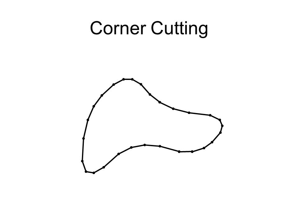
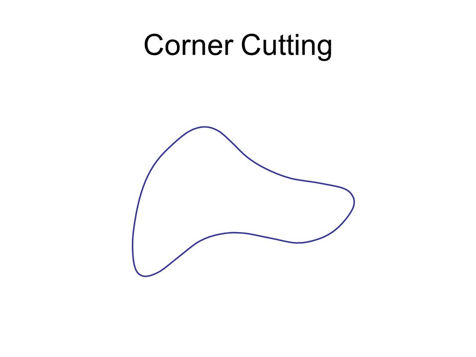
25 Corner Cutting

26 1 : 3 3 : 1

27 Corner Cutting

28

29

30

31

32

33 The control polygon The limit curve A control point

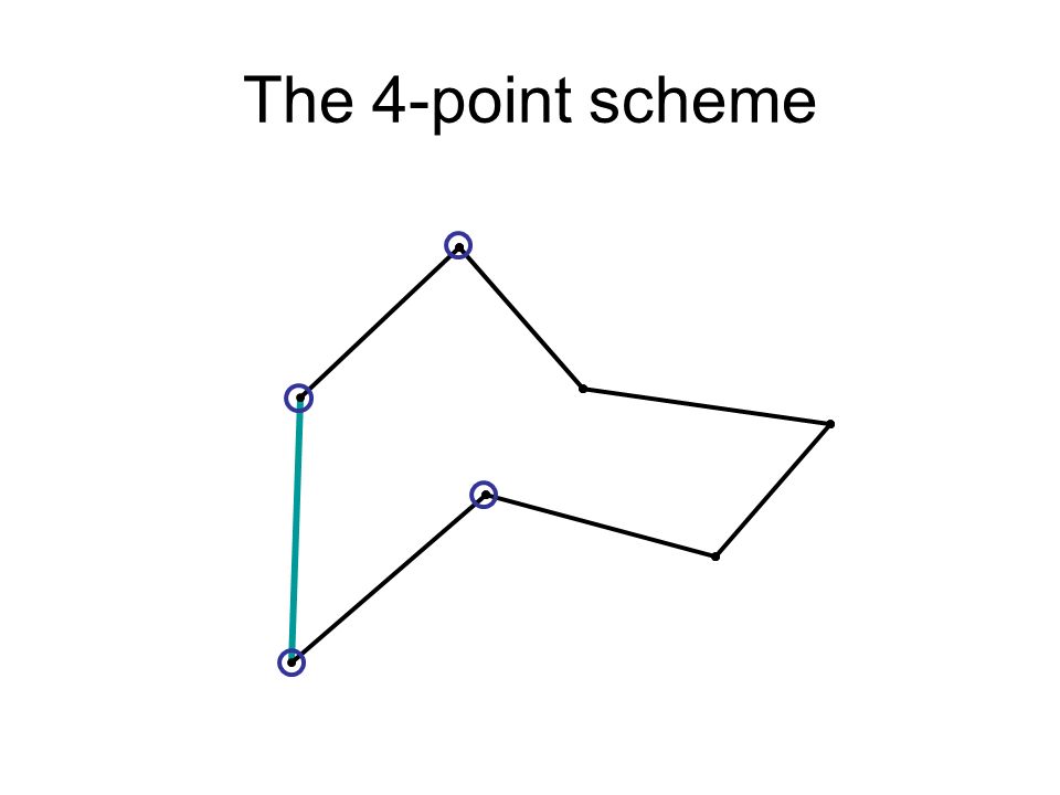
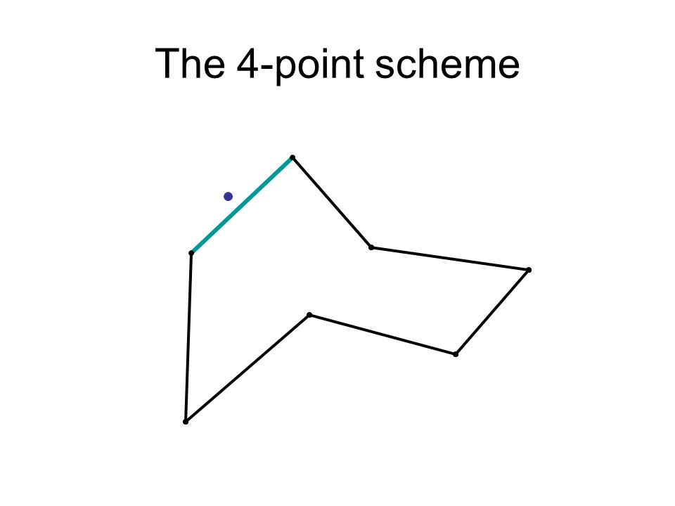
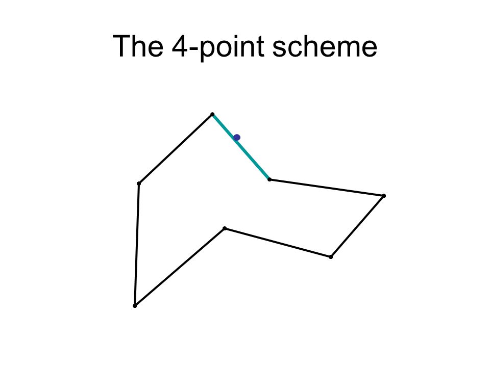
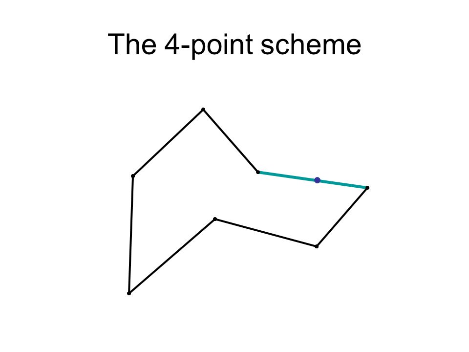
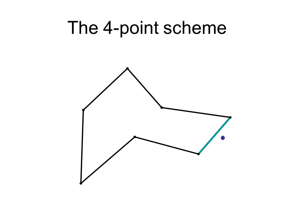
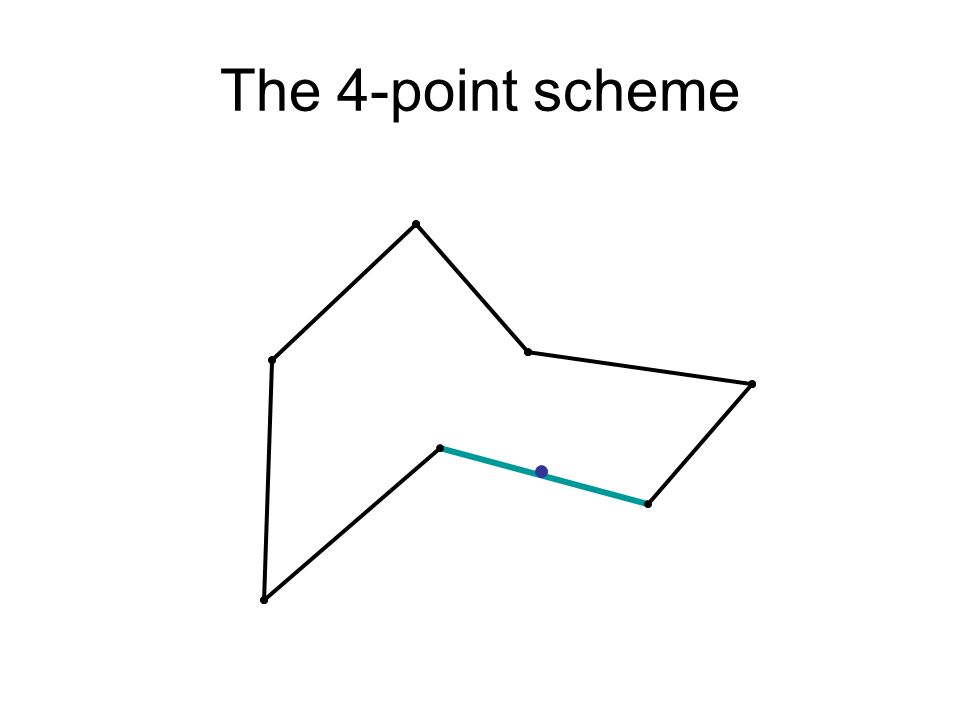
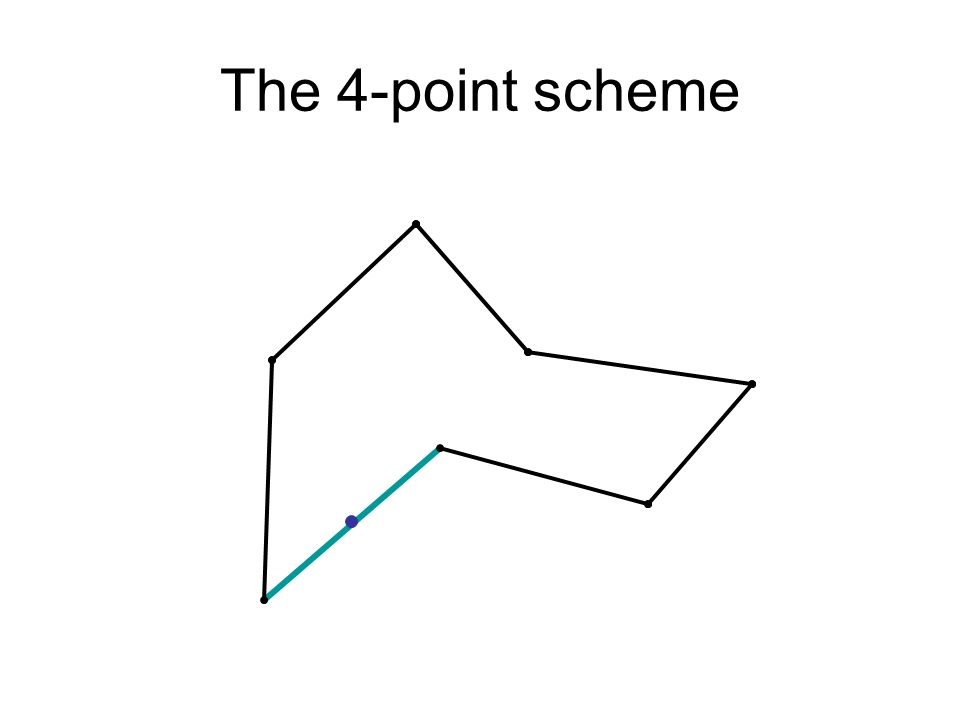
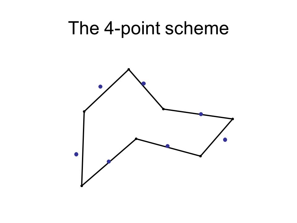
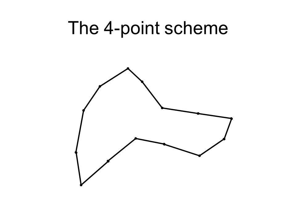
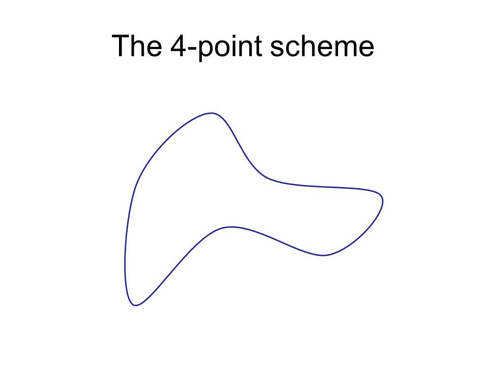
34 The 4-point scheme

35

36 1 : 1

37 The 4-point scheme 1 : 8

38 The 4-point scheme

39

40

41

42

43

44

45

46

47

48

49 The control polygon The limit curve A control point

50 Subdivision curves Non interpolatory subdivision schemes Corner Cutting Interpolatory subdivision schemes The 4-point scheme

51 Basic concepts of Subdivision A subdivision curve is generated by repeatedly applying a subdivision operator to a given polygon (called the control polygon). The central theoretical questions: –Convergence : Given a subdivision operator and a control polygon, does the subdivision process converge? –Smoothness : Does the subdivision process converge to a smooth curve?

52 Subdivision schemes for surfaces A Control net consists of vertices, edges, and faces. In each iteration, the subdivision operator refines the control net, increasing the number of vertices (approximately) by a factor of 4. In the limit the vertices of the control net converge to a limit surface. Every subdivision method has a method to generate the topology of the refined net, and rules to calculate the location of the new vertices.

53 Triangular subdivision Works only for control nets whose faces are triangular. Every face is replaced by 4 new triangular faces. The are two kinds of new vertices: Green vertices are associated with old edges Red vertices are associated with old vertices. Old vertices New vertices

54 Loops scheme 33 1 1 1 1 1 1 1 n - the vertex valency A rule for new red verticesA rule for new green vertices Every new vertex is a weighted average of the old vertices. The list of weights is called the subdivision mask or the stencil.

55 The original control net

56 After 1st iteration

57 After 2nd iteration

58 After 3rd iteration

59 The limit surface The limit surfaces of Loops subdivision have continuous curvature almost everywhere.

60 The Butterfly scheme This is an interpolatory scheme. The new red vertices inherit the location of the old vertices. The new green vertices are calculated by the following stencil: 8 8 2 2

61 The original control net

62 After 1st iteration

63 After 2nd iteration

64 After 3rd iteration

65 The limit surface The limit surfaces of the Butterfly subdivision are smooth but are nowhere twice differentiable.

66 Quadrilateral subdivision Works for control nets of arbitrary topology. After one iteration, all the faces are quadrilateral. Every face is replaced by quadrilateral faces. The are three kinds of new vertices: Yellowfaces Yellow vertices are associated with old faces Green vertices are associated with old edges Red vertices are associated with old vertices. Old vertices New vertices Old edge Old face

67 Catmull Clarks scheme 1 1 1 1 1 First, all the yellow vertices are calculated Step 1 1 1 1 1 Then the green vertices are calculated using the values of the yellow vertices Step 2 1 1 1 1 1 1 1 1 1 Finally, the red vertices are calculated using the values of the yellow vertices Step 3 n - the vertex valency 1

68 The original control net

69 After 1st iteration

70 After 2nd iteration

71 After 3rd iteration

72 The limit surface The limit surfaces of Catmull-Clarkss subdivision have continuous curvature almost everywhere.