Martin Handford, Where´s Wally? Parte IV – Integração de Dados Silvana Amaral Antonio Miguel V. Monteiro CST.

Apresentação em tema: "Martin Handford, Where´s Wally? Parte IV – Integração de Dados Silvana Amaral Antonio Miguel V. Monteiro CST."— Transcrição da apresentação:

1 Martin Handford, Where´s Wally? Parte IV – Integração de Dados Silvana Amaral Antonio Miguel V. Monteiro {silvana@dpi.inpe.br, miguel@dpi.inpe.br} CST 310: População, Espaço e Ambiente Abordagens Espaciais em Estudos de População: Métodos Analíticos e Técnicas de Representação 4. Métodos Dasimétricos

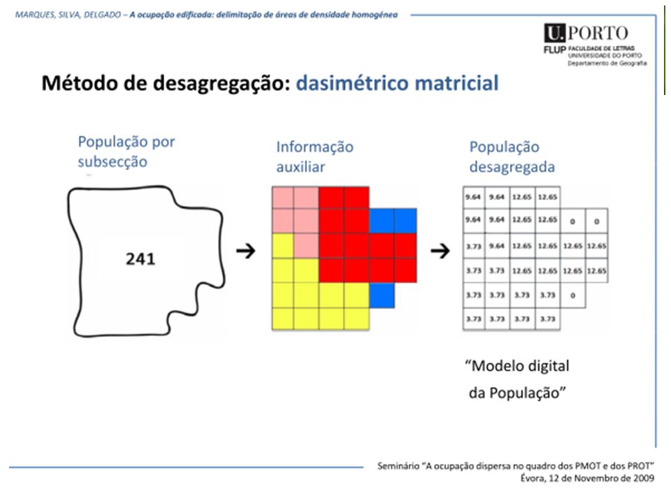
2 Origem dasymetry [física] s. dasimetria, f.; parte da Física que estuda a determinação da densidade do ar nas diferentes camadas da atmosfera Dasymetric map Criado por Benjamin (Veniamin) Petrovich Semenov-Tyan-Shansky e popularizado por Wright (1936). Dasymetric mapping may be defined as a kind of areal interpolation that uses ancillary (additional and related) data to aid in the areal interpolation process. IS NOT= to choropleth mapping: the boundaries of cartographic representation are not arbitrary but reflect the spatial distribution of the variable being mapped (Eicher and Brewer 2001).

3 Objetivos - aplicações –Suporte para elaboração de superfícies de densidade populacional –Levantamento de dados –Reconhecimento dos processos e sua heterogeneidade espacial –Interação com outros aspectos e interesses –Suporte para Modelagem

4 Aplicação Langford, 2007

5 Mapeamento Dasimétrico Silva, 2010

6 Mapeamento Dasimétrico Binário (MDB) Silva, 2010

7 Mapeamento Dasimétrico Binário (MDB) Silva, 2010

8 Mapeamento Dasimétrico Inteligente (MDI) Silva, 2009 Mennis e Hultgren 2006

9 Mapeamento Dasimétrico Inteligente (MDI) Silva, 2009

10 Aplicação

11

12

13 Exemplo didático… Perspectiva e Objeto de estudo Dinâmica Populacional e Assentamentos Humanos Geração de Território

14 Interações – População x Cobertura

15 DP & DPHA – Pensando Marabá Para entender mobilidade: –Núcleos urbanos - ocorrência e conectividade –Informações demográficas (migração) – INCRA, ONGs? –Estradas a acessos / vicinais –População ribeirinha –Indicadores das redes técnicas, físicas e sociais –Energia elétrica – produção e consumo (*)

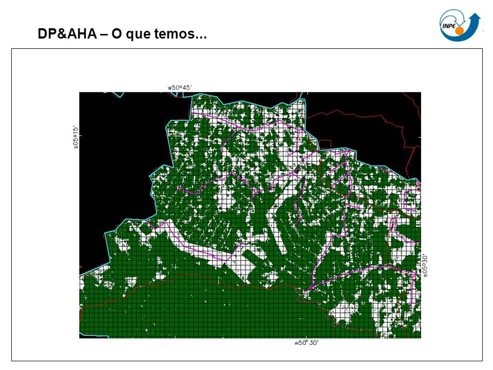
16 DP&AHA – O que temos... Marabá –15.137,4 km 2 município –População –Como encontra-se distribuída esta população?

17 DP&AHA – O que temos... Luzes Noturnas – Escala Global

18 DP&AHA – O que temos... Setores Censitários 2000 *

19 DP&AHA – O que temos... Setores Censitários 2000 * - Densidade Populacional

20 DP&AHA – O que temos... Setores Censitários 2000 * - Heterogeneidade

21 DP&AHA – O que temos...

22

23

24 Redistribuição de setores censitários para células Incluir heterogeneidade Setores Censitários de um município Considerações / Método –Água e floresta Restrição de células –Variáveis para indicar presença -> Superfície de população –Relação entre as variáveis -> Redistribuição População em Marabá Desagregando no município... Limites Poligonais Modelo Superfície Adjacente RedistribuiçãoPopulação em células

25 Imagens de satélite Classes Água e Floresta CBERS para região Landsat para município Técnicas simples de classificação digital Células 95% Método Dasimétrico

26 Operadores Média Simples Média Ponderada Fuzzy Mín, Máx e Gama Relação entre as variáveisPonderação setor Potencial de População Superfície AdjacenteVariáveis x População Valores médios Buffer distritos (PA) Função QuadráticaValores – Pertinência Fuzzy Método Multivariado Empírico / Literatura Distância Vias Distância Rios Distância Centros Urbanos Cobertura Florestal Declividade Seleção Variáveis Indicadoras Inferir superfície que descreva distribuição SR & SIGDados locais p/ variáveis

27 Método Multivariado – Contribuição relativa das variáveis preditoras Distritos do PA Área de Influência Média das distâncias a vias, distância a rios, declividade Distância a centros urbanos – Viz + Próx. Percentagem Floresta 5% < x < 99%

28 Classificação contínua ouA análise espacial em SIG será muito melhor realizada com uso da técnicas de classificação contínua: os dados são transformados para o espaço de referência [0,1] e processados por combinação numérica, através de média ponderada ou inferência “fuzzy” Isto nos permite construir cenários (por exemplo, risco de 10%, 20% ou 40%), que indicam os diferentes compromissos de tomada de decisão => maior flexibilidade e um entendimento muito maior sobre os problemas espaciais Lógica Fuzzy: Introduzida por Lofti Zadeh (1960s), como um meio de modelar incertezas da linguagem natural Lógica Fuzzy é uma extensão da lógica Booleana: “verdade parcial”, valores entre “completamente verdadeiro” e “completamente falso” 0 1 Falso Verdade Lógica Boleana z F V F(z) Lógica Fuzzy z V F 0 1 Falso Verdade

29 29 Conjuntos Fuzzy Exemplo: Altura de Pessoas –S um conjunto fuzzy ALTO, que responderá a pergunta: " a que grau uma pessoa “z” é alta? Z : S = (z, f(z)) especialistas 0 1 BAIXO ALTO z f(z) 1.52.1 0.5 Exemplo: ”João é ALTO" = 0.38          1.2,1 1.25.16.0/)5.1( 5.1,0 )( zse z z z zf

30 30 Conjuntos Fuzzy Outro exemplo - Declividade f (z) = 0 se z   f(z) = 1/[1+  (z  ) 2 ] se  < z <  f(z) = 1 se z   0 0.2 0.4 0.6 0.8 1 0.025 40 Declividade Mínimo (  ) Máximo (  ) f(z) = f(z) = 0 se z  0.025 f(z) = f(z) = 1/[1+ 0.025(z  40) 2 ] se  < z < 40 f(z) = f(z) = 1, se z  40

31 Variáveis preditoras Parâmetros

32 Método Multivariado – Função de Pertinência Fuzzy

33 Método Multivariado – Variáveis indicadoras Mapas Distância Rios Distância Estradas Distâncias setores urbanos Classificação Floresta e água D Setores Urbanos D Estradas D Rios

34 Método Multivariado – Variáveis indicadoras Mapas Distância Rios Distância Estradas Distâncias setores urbanos Classificação Floresta e água D Setores Urbanos D Estradas D Rios

35 Método Multivariado – Variáveis indicadoras Mapas Distância Rios Distância Estradas Distâncias setores urbanos Classificação Floresta e água D Setores Urbanos D Estradas D Rios

36 Método Multivariado – Variáveis indicadoras Mapas Distância Rios Distância Estradas Distâncias setores urbanos Classificação Floresta e água F (Z) Mundo Celular...

37 Método Multivariado – Variáveis indicadoras Mapas (F(z)) Declividade Distância Rios Distância Estradas Distâncias setores urbanos Classificação Floresta e água E como estas variáveis podem resultar em um valor de possibilidade de ocorrência de população???

38 Inferência Fuzzy Dados em conjuntos Fuzzy manipulados com métodos lógicos da lógica fuzzy ou operadores fuzzy AND, OR, Soma algébrica, Produto Algébrico, Operador Gama e Soma Convexa OR (otimista) res = MAX (crit1, crit2, …) AND (pessimista) res = MIN (crit1, crit2, …) Produto Algébrico res =  (crit1,crit2,..) Soma Agébrica res = 1 -  (crit1,crit2,..) Operador Gama (compromisso) res = [soma algébrica (crit1, crit2, …)]  * [produto algébrico (crit1, crit2, …)] 1- 

39 Método Multivariado – Variáveis indicadoras Mapas (F(z)) Declividade Distância Rios Distância Estradas Distâncias setores urbanos Classificação Floresta e água

40 Método Multivariado – Variáveis indicadoras E a distribuição da população / célula???? Onde: DP grid é a densidade demográfica da célula, P CS é a população do setor censitário, F grid é o valor Fuzzy de possibilidade de ocorrência de população para a célula ponderado pela somatória dos valores Fuzzy obtidos para o setor censitário e considerando-se apenas as células válidas, ou seja, com percentagem de floresta e corpos d’água maior que 95%.

41 Operadores Média Simples Média Ponderada Fuzzy Mín, Máx e Gama Relação entre as variáveisPonderação setor Potencial de População Superfície AdjacenteVariáveis x População Valores médios Buffer distritos (PA) Função QuadráticaValores – Pertinência Fuzzy Método Multivariado Empírico / Literatura Distância Vias Distância Rios Distância Centros Urbanos Cobertura Florestal Declividade Seleção Variáveis Indicadoras Inferir superfície que descreva distribuição SR & SIGDados locais p/ variáveis

42 População em Marabá Redistribuição – Superfícies resultantes - Região Restrição floresta e água ineficiente Percurso de campo Média Simples – mais variabilidade Média Ponderada superfície mais suave

43 População em Marabá Redistribuição – Superfícies resultantes - Região Fuzzy Mínimo representou melhor a heterogeneidade espacial

44 População em Marabá Redistribuição – Superfícies resultantes – Município

45 População em Marabá Redistribuição – Superfícies resultantes – Município

46 População em Marabá Redistribuição – Superfícies resultantes – Município

47 População em Marabá Redistribuição – Superfícies resultantes – Município

48 População em Marabá Redistribuição – Superfícies resultantes – Município

49 População em Marabá Redistribuição – Superfícies resultantes – Município

50 População em Marabá Redistribuição – Superfícies resultantes – Município

51 População em Marabá Redistribuição – Superfícies resultantes – Município Restrição floresta e água – setores sem população Média Simples – mais variabilidade que Média Ponderada (peso para % floresta) Fuzzy Mín e Gama similares Fuzzy Máx semelhante Setores com restrição inicial Dados de pessoas nos PAs do INCRA para análise global Fuzzy gama – acertos nas classes de densidade extremas Média Simples – acerto nas classes intermediárias

52 Método Dasimétrico x Acesso a Saúde Measuring Potential Access to Primary Healthcare Services: The Influence of Alternative Spatial Representations of Population Mitchel Langford; Gary Higgs This article studies the implications of adopting differing spatial representations of population on healthcare accessibility modeling outcomes.

53 Langford & Higgs (2010) Motivation (National Health Service) Priorities and Planning Framework 2003–2006 reduction in health inequality GIS - identifying poorly served areas through combinations of data relating to sociodemographic circumstances, supply/demand characteristics, and appropriate transportation information. Context Traditional approaches to measuring geographical barriers to health services: potential accessibility: concerned with opportunities available to residents within administrative areas generally realized accessibility: on utilization data (e.g., postcoded patient lists, referral and/or attendance records, and actual travel behavior) that permit measures of accessibility to be directly calculated.  developed potential measures of access based on either straight-line or travel-time distances between health services and demand points.  Such measures are then used to identify areas where provision is poor and where additional health facilities are needed to improve levels of access

54 Langford & Higgs (2010) Ex: Development Agency report (2004), for example, found that over 10 percent of households in rural areas outside the South East of England were more than seven miles (11.26km) from their nearest hospital. Studies have compared the relative utility of both approaches in association with socioeconomic characteristics of areas, often with contrasting findings. Individuals attend the nearest facility there is no cross-boundary flow of patients Some research into the impacts of using different GIS-based techniques on resultant accessibility measures (e.g., Brabyn and Barnett 2004),  but other confounding factors have received little focus, one such issue being the estimation of potential population demand

55 Langford & Higgs (2010) Traditionally the total population (or relevant subgroups) potentially able to access health facilities is derived by computing Euclidean or drivetime catchments around healthcare delivery points An estimated population count is then obtained using spatial interpolation techniques. –point-in-polygon analysis location-allocation modeling, and previous work has explored potential im plications of generalizing demand at a single point with potential location uncertainties (e.g.,Hewko, Smoyer-Tomic, and Hodgson 2002). – areal interpolation tools counting only those census tracts entirely enclosed within the catchment, or including those that only partially intersect the catchment, or including the population of partially intersecting tracts on a pro rata basis determined by the area of overlap. The population assignment technique chosen inevitably impacts on estimates of those deemed to be with-in reach of health facilities and Each method has limitations we ignore populations in tracts not completely bounded by the travel catchment we are assuming equal distribution of population within census tract allocating(or not) the entire population of a tract on the basis of just one representative point.

56 Langford & Higgs (2010) Specifically we are concerned with comparing demand-side measures based on areal interpolation by dasymetric mapping with those derived from more established approaches. Researchers are largely concerned with variations in availability of service rather than the relationship between availability and service utilization. !!

57 Langford & Higgs (2010) Researchers are largely concerned with variations in availability of service rather than the relationship between availability and service utilization. !! Geographical availability of services (Kernel density estimates- KDE) X Population need – (population-tract centroids - health record based on the mother’s census tract of residence) OBS: USA – Urban area – no travel distance In the absence of individual-level health data, measures are often based on a count of services within census tracts or, alternatively, the number of facilities within a certain Euclidean distance or drive-time of single demand points

58 Langford & Higgs (2010) - methodology Uses adaptation of the two-step floating catchment area method, Spatial representation models of the population: 1. population–weighted centroid (Office for National Statistics- ONS) 2. evenly distributed within the census tabulation zone OR ‘‘areal weighting’’ 3. dasymetrically distributed with in the census tabulation zone. create subzones of relative homogeneity and thereby ensure that mapped discontinuities better reflect the true underlying geography. - lacks a standardized methodology and variations are possible in terms of the choice of ancillary data used or the degree of internal differentiation attempted - USED two-tier, binary dasymetric method; -internally mapping each census tabulation zone into subareas identified as either occupied or empty, then allocating the population count uniformly to only the occupied portion. -

59 Langford & Higgs (2010) - methodology Ancillary data: Ordnance Survey (OS, the U.K. national mapping agency) 1:50000 scale raster maps: (geotiff, 5m) - full U.K. coverage and carries details of roads, footpaths, woods, water features buildings, and contour heights - Binary : white  populated areas

60 Langford & Higgs (2010) - methodology Population representations

61 Langford & Higgs (2010) - methodology To evaluate the impacts of these models healthcare services within Wales was assembled: 2,010 GPs distributed across 485 practices, geocoded to point locations using the NHS postcode directory,

62 Langford & Higgs (2010) - methodology Travel-time catchments were computed using a road network the vector road network, clipped to the Welsh national boundary, was rasterized to a grid with a 25-m posting. The final result was a travel cost raster from which a travel-time catchment could be computed for any designated location using any specified threshold time limit. Travel-time catchments, using a 10- minute threshold, were computed for each GP practice in turn using the CostAllocation function

63 RESULTS A dasymetric representational model leads to higher estimates of the floating catchment population  physician availability is always somewhat lower than might previously have been thought Langford & Higgs (2010) – methodology/results corresponding physician-to-population ratios (i.e., Rj). VBA (Visual Basic for Applications) script that cycled through each GP practice in turn, computing travel-time catchments and performing raster overlays with each population surface to determine the Rj values. Rj values. assigned to GP point objects via their attribute tables. The sum total of Rj values contained within that zone yields thefinal accessibility index (Af )

64 Langford & Higgs (2010) - results Absolute difference in accessibility scores for the Cardiff Unitary Authority between the dasymetric and pro rata population distribution models. Accessibility scores (Af ) plotted for Output Areas in the Cardiff Unitary Authority (representative point population distribution model and ten- minute travel time threshold).

65 Langford & Higgs (2010) – Results Af patterns they exhibit over space help to identify isolated pockets of impoverished healthcare accessibility. Difference: the discrepancy between models increases as rurality increase. a clear tendency for larger, less-urbanized Output Areas lying beyond the city limits to report the greatest decline in Af score when comparing these two representational models of population dasymetric model was found to consistently yield proportionately lower estimates of healthcare accessibility (using the floating catchment technique) in rural as compared to urban regions. The dasymetric representation is believed to provide the most detailed and realistic understanding of population geography within census tract boundaries, and therefore should offer the best estimates of potential demand on services.

66 PCI & Maxent Bajat B., Hengl, T., Kilibarda,M. & Krunic, N. Mapping population change index in Southern Serbia (1961–2027) as a function of environmental factors. Computers, Environment and Urban Systems 35 (2011) 35–44 using a maximum entropy model (MaxEnt software) and publicly available environmental layers for modeling of population change index (PCI). Aim: determine the habitat suitability index (HSI), commonly used in ecology, and then use this index to try to explain population dynamics, i.e. the population change index (PCI) expressed as the population ratio between various periods. Assumption: will be able to explain spatial pattern of population dynamics by using environmental and demographic factors and by following the Niche analysis methods that have been shown efficient in explaining distribution of plant and animal species in ecology.

67 PCI & Maxent PCI - the ratio of change in the number of inhabitants at certain location for an observed period between two censuses P1 = pop time ini P2 = pop time end observed period 0 < PCI <  - study case 0 – 6.32 (632% ), as the distribution of values will be skewed because the spatial distribution of population typically follows the Poisson  Adjusted PCI (normal) Fig. 1. Scheme showing actual distribution of population density for two periods. The smoothed line represents the deterministic part of variability that can often be explained by using environmental and socio-economic factors.

68 PCI & Maxent PCI - try to explain it using various environmental and socio-economic factors: q are the environmental predictors (topography, proximity to work and cultural centers, land cover, proximity to leisure activities and similar), available for given time period t, at locations s (s {xi, yi}), and  is the error term. Variation in the values contains deterministic (smooth) component and some residual that can possibly be explained by spatial proximity (or cannot be explained at all)data = smooth + rough or P* is the deterministic part,  is the residual term Interest: the smooth or the deterministic part of variation in PCI values (smoothed line Fig.1)

69 Maxent Modelagem de Distribuição Geográfica de Espécies Maxent Distribuição de probabilidade potencial para toda área (soma dos pixels =1) Modelagem de Distribuição Geográfica de Espécies Distr Prob ? Elisangela S. C. Rodrigues, 2010

70 Maxent Entropia é uma medida de desordem ou previsibilidade de um sistema. É uma medida de incerteza de um acontecimento. Observacoes inesperadas tem mais informação que observações esperadas Está relacionada à probabilidade de ocorrência de um evento: Quanto maior a probabilidade de ocorrer um evento, menor a entropia. Se P for alta, nao vai ter info associada. Vai ser uma surpresa! Vai trazer informação! Entropia máxima: P uniforme (dado não viciado), Se o dado for viciado, a entropia vai ser menor, pq a P será maior. Incerteza → surpresa → informação (entropia no acontecimento de um evento, ou incerteza) Elisangela S. C. Rodrigues, 2010

71 Maxent Princípio da Entropia Máxima: Tendo-se varias distribuições de probabilidade possíveis deve-se escolher a distribuição de probabilidade cuja a entropia é máxima (mais dispersa ou próxima da uniforme) de acordo com algumas restrições. Entropia: quantidade de incerteza na ocorrência de algum evento. Associado a quantidade de informação transmitida no evento (“métrica”) Tendo-se várias distribuições de probabilidade possíveis para aquele conjunto de pontos e camadas, deve-se selecionar aquela distribuição que transmita o maior quantidade de informação possível => Entropia Máxima Distr Prob ? Elisangela S. C. Rodrigues, 2010

72 Maxent Restrições => representam as evidências, ou seja, fatos conhecidos sobre o conjunto de dados de entrada, neste caso são as camadas ambientais.(features) X => região geográfica de interesse x1, x2,...,xn => ptos observados/registrados f1, f2,...,fn => features (valor da camada ou uma função do valor de entrada ) Tarefa: Tendo conjunto de pontos e de camadas, tem-se que encontrar a distribuição de probabilidade para este conjunto de dados: Restrições: –Features, evidências (critério sobre os valores das camadas) –Soma das prob = 1. xn x1 x2 x3 x4 n distribuições de probabilidade possíveis Elisangela S. C. Rodrigues, 2010

73 Maxent Existem várias distribuições de probabilidade que satisfazem todas as restrições. Quando isso acontece, o modelo é considerado consistente e dentre estes, tem-se que escolher aquele q tem a entropia máxima (p *) Encontrar os pesos para cd uma das features de forma q o resultado seja de Max entropia x1 x2 x3 x4 xn O modelo expressa a adequação de cada célula da grade como uma função das variáveis ambientais daquela célula. Um valor alto desta função numa célula indica que ali existem condições favoráveis para a espécie. Predição de condições favoráveis Do modelo, faz-se a projeção para a área, usando as variáveis ambientais http://www.cs.princeton.edu/~schapire/maxent/

74 PCI & Maxent Serbia population -Census data for years 1961 and 2002 (Statistical Office of the Republic of Serbia, 2003), polygon map with table data - Population counts for year 2027 were estimated by using the analytical method of components

75 PCI & Maxent Dasymetric method for resolution downscale (200m) It assumes that each source zone (census unit) contributes to the target zone with a portion of its data proportional to the percentage of its area that the target zone occupies. Pj is the estimated population of target zone j; Atsp is the area of overlap between target zone t and source zone s, and having land cover identified as populated; Ps is the population of source zone s; Adsp is the area of source zone s having land cover identified as populated; S is the number of source zones, dsp is the dasymetric density of the populated class in source zone s (boundaries of settlement polygons (749 built-up areas) digitized from 1:100 k topo map and then split each source zone into populated and uninhabited) ! procedure described above satisfies pycnophylactic property of areal interpolation  Sum population total maintained.

76 PCI & Maxent Auxiliary maps - GIS layers to model the population change: SRTM_DEM – SRTM based digital elevation model. TWI – Topographic wetness index derived using the 90 m DEM and resampled to 200 m grid. Slope – Slope map derived using the 90 m DEM and resampled to 200 m grid. Dist1 – Buffer distance map based on category I roads. Dist2 – Buffer distance map based on category II roads. EVI2002 – Mean annual MODIS enhanced vegetation index for year 2002. IGBP2002 – MODIS land cover product map for year 2002.

77 PCI & Maxent R The dasymetric downscaling was implemented in R by combining the merge and aggregate methods. After we downscale population counts to 200 m grid, we can derive the PCI using Eq. (2) and then can correlate it with environmental predictors. In R syntax: PCI.lm is is the resulting linear regression model object. We compare this model to Maxent using only derived HSI as predictor Note also that we basically use all grid nodes (grids200m@data) in the map to fit the model, so that the resulting model aims at depicting the mean deterministic component of the signal (smooth part ). This pattern would otherwise not be visible from the original polygon data.

78 PCI & Maxent Results - higher spatial accuracy of the map, and more realistic distribution of the population 1961 and 2027

79 PCI & Maxent Environmental variables - TWI and DEM greatest contribution x Processes in the area: the main vectors of migration can be connected with people moving from villages in the highlands to urban agglomerations in the valleys. -High EVI (indicating dense vegetation/forests) and land cover classes seem to be of low relevance. -TWI is the environmental variable with the highest gain when it is used isolated. At the same time TWI most decreases the gain when it is omitted, which means that TWI contains most of information that are not immanent in other variables.

80 PCI & Maxent Maxent - suitable habitat index (HSI) for both periods. Green shades of color indicate high inhabiting preference and red colored areas indicate low preference.  mainly a function of topography

81 The results of linear regression/correlation analysis using the derived PCI and the environmental variables (Dist1, Dist2, TWI, IGBP2002, Slope, SRTM_DEM) show that these predictors can explain up to 40% of variation in PCI values. Regression analysis between PCI and HSI2027 explains 29% of variation in PCI. Population change and inhabiting preference are interconnected concepts, but the original predictors are more suited for spatial prediction of PCI. PCI & Maxent

82 The predicted results were also verified with real population distribution data. The modeled PCIm values for the period 1961–2002 were predicted by environmental predictors These values were used afterwards to predict modeled population distribution for year 2002, Pm(2002): The modeled map of Pm(2002) was compared with corresponding P(2002) map The correlation coefficient obtained was r = 0.930, indicating the great level of agreement among modeled and real population distribution data. -The resulting pattern in the derived PCI map also coincides with our expectations (see previous section): the population migration mainly follows the pattern of main road networks. -Roads are the main attractor of new inhabitants. PCI & Maxent

83 Remarks -inhabiting preference (HSI) for year 1961 is mainly a function of topography (TWI, elevation). -population growth can be connected with low and flatlying landscapes, and with proximity to road networks -Distribution of population is distinctly controlled by environmental factors with an AUC > 0.84 (cross-validation), which indicates that the model is highly accurate. - The advantage of using environmental predictors to explain population dynamics is that it enables us to prove and visualize spatial correlation between the two features -Environmental grids Dist1, Dist2, IGBP200212 (croplands), IGBP200213 (urban/built areas), EVI2002 were able to explain 40% of variability in the population change index. -For comparison,HSI (year 2027) explains 29% of variability in PCI with a curved relationship. -This indicates that, although conceptually similar indices, there is still a difference between the HSI (preference) and PCI (migration). Demographic changes were solely considered from the aspect of inhabiting preferences. We did not consider political and socio-economical aspects of the Region such as distance to main industrial sites and markets and amenities, that were not available in this case -We also did not even try to model the residual part in Eq. (3). PCI & Maxent

84 Referências Wright, John K. 1936. A method of mapping densities of population with Cape Cod as na example. Geographical Review 26:103–10. Teresa Sá Marques, R.S.; Silva, F.B.; Delgado C. A ocupação edificada: delimitação de áreas de densidade homogénea. Departamento de Geografia, FLUP / CEGOT <http://repositorio-aberto.up.pt/handle/10216/19849http://repositorio-aberto.up.pt/handle/10216/19849 Filipe Batista e Silva. 2009. Modelação cartográfica e ordenamento do território: um ensaio metodológico de cartografia dasimétrica aplicado à região oeste e Vale do Tejo. Dissertação de Mestrado. Faculdade de Letras da Universidade do Porto http://repositorio-aberto.up.pt/handle/10216/18045http://repositorio-aberto.up.pt/handle/10216/18045 Langford, Mitchel and Higgs, Gary(2006) 'Measuring Potential Access to Primary Healthcare Services: The Influence of Alternative Spatial Representations of Population', The Professional Geographer, 58: 3, 294 — 306. DOI: 10.1111/j.1467-9272.2006.00569.x. http://dx.doi.org/10.1111/j.1467- 9272.2006.00569.x Bajat B., Hengl, T., Kilibarda,M. & Krunic, N. Mapping population change index in Southern Serbia (1961–2027) as a function of environmental factors. Computers, Environment and Urban Systems 35 (2011) 35–44