AC-723 – MÉTODOS EXPERIMENTAIS PARA TURBINA A GÁS –

Apresentação em tema: "AC-723 – MÉTODOS EXPERIMENTAIS PARA TURBINA A GÁS –"— Transcrição da apresentação:

1 AC-723 – MÉTODOS EXPERIMENTAIS PARA TURBINA A GÁS –
aulas 24-27 Prof.(a) Cristiane Martins Instituto Tecnológico de Aeronáutica Divisão de Eng. Aeronáutica / Dept. de Propulsão 10/2010

2 Mapa do Curso Introdução ao LabVIEW Arrays, Graphs, & Clusters
Criar, Editar, & Debugar uma VI Local Variable & Property Node Case & Sequence Structures e Formula Nodes Criar SubVI Page SG-10: Give a rough time frame of topics to be covered: Day 1 - Introduction to LabVIEW Creating, Editing, and Debugging a VI Creating a SubVI Loops and Charts Day 2 - Arrays and Graphs Case and Sequence Structures Strings and File I/O Day 3 - (Find out if anyone is leaving early on the last day. If so, you may need to switch the order of the last two chapters.) VI Setup Instrument Control Data Acquisition Data Acquisition & Waveforms Loops & Charts Strings & File I/O Projeto VI

3 Introdução ao LabView Semana 11–aula 11 Revisão – Assunto a tratar
PROJETO AQUISIÇÃO DE DADOS

4 Projetos - Cada grupo deverá fazer apresentação em classe dos passos e da VI construída. Todos os projetos serão testados no Laboratório. Três projetos – dois com maior dificuldade. Seleção dos alunos foi de acordo com a dificuldade do projeto – alunos com maior facilidade projetos com maior dificuldade.

5 Projeto 1 – Motor Foguete
Parte 1 – Previsão de comportamento do motor Parte 2 – Aquisição de dados

6 Projeto 1 – Motor Foguete
Frederico Della Bidia Bruno Goffert André Fernando Ana Maria Lincoln Tolomelli

7 Projeto 2 – Turbina a Gás Parte 1 – Aquisição de dados
Parte 2 - Controle da turbina

8 Projeto 2 – Turbina a Gás Eduardo Maiello Bruno Machado Bruno Goulart
Jocicley Jamaguiva Alexandre Damião

9 Projeto 3 – Temperatura estática
Parte 1 – Equacionar o problema Parte 2 – Aquisição de dados

10 Projeto 3 - Temperatura estática
Daniel Yiuji Lina Augusta Juliana Mara Andrei Silva Souza

11 Planejamento e Projeto Processo
Topo - abaixo Base- subida Definir Projeto Feedback Teste & Ajuste Final Fluxograma Integrar SubVIs no Projeto Page 1-2 This is one possible design approach, and is not intended as a general solution. Discuss the steps in this design process: Clearly define project goals and system requirements. Design a flowchart for the application. Implement nodes in the flowchart as subVIs where possible. By creating a hierarchical set of VIs, you can find and fix bugs more quickly during testing. After the individual components work, begin integration into the larger project. Test the final product and release it. Use customer feedback and updated design goals to improve the product. Implementar Nodes como VIs Teste SubVIs

12 Arquitetura Simples VI
VI que produz resultados quando roda Nenhuma opção de “start” ou “stop” Adequado para testes de lab, cálculos Exemplo: Convert C to F.vi You can structure VIs differently depending on what functionality you want them to have. This section discusses some of the most common types of VI architectures, along with their advantages/disadvantages: simple, general, parallel loops, multiple cases, and state machines. For a more complete discussion of the types of VI architectures, see the presentation entitled “Techniques for Large Application Development in G” by Gregg Fowler and Stepan Riha from the 1998 NIWeek proceedings. Simple VI Architecture When making quick lab measurements, you do not need a complicated architecture. Your program may consist of a single VI that takes a measurement, performs calculations, and either displays the results or records them to disk. The measurement can be initiated when the user clicks on the run arrow. In addition to being commonly used for simple applications, this architecture is used for “functional” components within larger applications. You can convert these simple VIs into subVIs that are used as building blocks for larger applications. The example shown above is the Convert to dB VI you built in Exercise This VI performs the single task of converting a voltage array to dB. You can use this simple VI in other applications that need this conversion function without needing to remember the equation.

13 Arquitetura Geral VI Três passos principais Startup Main application
General VI Architecture In designing an application, you generally have up to three main phases: * Startup—Use this area to initialize hardware, read configuration information from files, or prompt the user for data file locations. * Main Application—Generally consists of at least one loop that repeats until the user decides to exit the program, or the program terminates for other reasons such as I/O completion. * Shutdown—This section usually takes care of closing files, writing configuration information to disk, or resetting I/O to its default state. The diagram above shows this general architecture. Notice that this resembles the diagram you build for the Freq Response VI. The startup procedure for the Freq Response VI initialized the function generator and the multimeter and calculated the frequency increment between steps. The main application consisted of sending a sine wave of the correct frequency from the function generator, reading the circuit response from the multimeter, doing the mathematical calculations, and plotting the results. The shutdown procedure consisted of closing the instruments and checking for errors. For simple applications, the main application loop can be fairly straightforward. When you have complicated user interfaces or multiple events (user action, I/O triggers, and so on), this section can get more complicated. The next few slides show design strategies you can use to design larger applications. Três passos principais Startup Main application Shutdown

14 Arquitetura com Loops Paralelos
Vantagens Manuseio simultâneo de processos múltiplos independentes Parallel Loop VI Architecture One way of designing the main section of your application is to assign a different loop to each event. For example, you might have a different loop for each action button on your front panel and for every other kind of event (menu selection, I/O trigger, and so on). This structure is straightforward and appropriate for some simple menu type VIs where a user is expected to select from one of several buttons that lead to different actions. This VI architecture also has an advantage over other techniques in that taking care of one event does not prevent you from responding to additional events. For example, if a user selects a button that brings up a dialog, parallel loops can continue to respond to I/O events. The main disadvantages of the parallel loop VI architecture lie in coordinating and communicating between different loops. The stop button for the second loop in the above diagram is a local variable. You cannot use wires to pass data between loops, because that would prevent the loops from running in parallel. Instead, you have to use some global technique for passing information between VIs. You can easily create “race conditions” where multiple tasks attempt to read and modify the same data simultaneously, which lead to inconsistent results and are difficult to debug. Global variables, local variables, and race conditions are discussed further in the LabVIEW Basics II course. Desvantagens Sincronização Troca de dados

15 Arquitetura com Multiplos ‘Cases’
Vantagens Sincronização e troca de dados simplificadas Desvantagens Loop pode ser grande demais e dificultar visualização Manuseio de um evento pode bloquear outros eventos Todos os eventos são manuseados a mesma taxa Multiple Case Structure VI Architecture The diagram above shows how to design a VI that can do multiple events that can easily pass data back and forth. Instead of using multiple loops, you can use a single loop that contains separate case structures for each event handler. This VI architecture would also be used in the situation where you have several buttons on the front panel that each initiate different events. The FALSE cases above are empty. An advantage of this VI architecture is that you can use wires to pass data. This helps improve readability. This also reduces the need for using global data, and consequently makes it less likely that you will encounter race conditions. Several disadvantages exist to the multiple case structure VI architecture. First, you can end up with diagrams that are very large and consequently are hard to read, edit, and debug. In addition, because all event handlers are in the same loop, each one is handled serially. Consequently, if an event takes a long time, your loop cannot handle other events. A related problem is that events are handled at the same rate because no event can repeat until all objects in the While Loop complete. In some applications, you might want to set the priority of user interface events to be fairly low compared to I/O events.

16 Arquitetura Máquina de Estado ‘State Machine Architecture’
States: 0: Startup 1: Idle 2: Event 1 3: Event 2 4: Shutdown State Machine VI Architecture You can make your diagrams more compact by using a single case structure to handle all of your events. In this model, you scan the list of possible events, or states, and then map that to a case. For the VI shown above, the possible states are startup, idle, event 1, event 2, and shutdown. These states are stored in an enumerated constant. Each state has its own case where you place the appropriate nodes. While a case is running, the next state is determined based on the current outcome. The next state to run is stored in the shift register. If an error occurs an any of the states, the shutdown case is called. The advantage of this model is that your diagram can become significantly smaller (left to right), making it easier to read and debug. One drawback of the Sequence structure is that it cannot skip or break out of a frame. This method solves that problem because each case determines what the next state will be as it runs. A disadvantage to this approach is that with the simple approach shown above, you can lose events. If two events occur at the same time, this model handles only the first one, and the second one is lost. This can lead to errors that are difficult to debug because they may occur only occasionally. More complex versions of the state machine VI architecture contain extra code that builds a queue of events (states) so that you do not miss any events. In the next exercise, you open and examine the state machine architecture VI shown in the slide above. The LabVIEW Basics II course describes state machines in more detail. Vantagens Pode ir para qualquer estado a partir de um outro Fácil de modificar e debugar Desvantagens Pode perder eventos se ambos ocorrem ao mesmo tempo

17 State Machine Cada estado em um ‘State Machine’ faz algo único e chama outros estados. Estado de comunicação depende de alguma condição ou sequência. Para variar o diagrama de estado no LabVIEW, preciso as seguintes infraestruturas: While loop – continuamente executa os vários estados Case structure – cada caso contém código a ser executado para cada estado Shift register – contém informação de estado de transição Transition code – determina o próximo estado na sequência

18 Um diagrama de estados representa um estado de máquina
Um diagrama de estados representa um estado de máquina. Estados de um estado de máquina são ativos ou passivos. Somente um estado está ativo em determinado tempo. O estado de máquina sempre parte de um estado particular definido como estado inicial e finaliza (pára) após o estado final.

19 Associado com um estado pode existir uma ou mais ações
Associado com um estado pode existir uma ou mais ações. Uma ação pode ser uma ação de controle executada por um controlador. Ações podem ser listadas como abaixo: Estado 1 ações: Acão 1: Valvula V1 is open; Acão 2: Motor M1 runs; Estado 2 ações: Ação 1: Valvula V1 is closed; Ação 2: Aquecedor H1 is on;

20 Ações para dado estado pode ser listadas em uma caixa fixada ao simbolo do estado, como mostra a Fig. ou de forma mais detalhada, dependendo da complexidade do programa.

21 Máquina de estado é uma estrutura conveniente do LabVIEW onde uma case construct where a case structure está contida em while loop. Execução de cases (em particular) na estrutura é determinada pela saída proveniente de um of particular cases in the structure is determined by the output from the previous case (or in the instance of the first execution) by the control selector input. Controle da ordem de execução de case é através do uso de shift register. The control of the order of case execution is controlled through the use of a shift register. By wiring the output from one case as the determinate to the subsequent case (wiring to the shift register on the right hand side) and wiring the input to the case selector from the left hand side shift register, operations can be ordered according to which state is executed.

22 Exercise 1-3 on Page Students examine the Timed While Loop and State Machine template VIs Approximate time to complete: 20 min. Pages 1-4 to 1-5: Please note any common questions and the approximate time required for this exercise, and return the information to the customer education department. We will update the manual accordingly.

23 RESUMO O processo de construção de uma aplicação pode ser dividido em três fases — planejamento, implementação e testes Ao planejar, assegure que máxima informação possível sobre a aplicação Faça fluxogramas Planeje a hierárquia de seu projeto Implemente sub componentes com subVIs onde for possível Desenvolva cada subVI e teste Combine todas as subVIs na aplicação completa Use técnica de masuseio de erros As arquiteturas mais comuns de VIs são Simples, Geral, Parallel While Loops, Multiple Cases, e State Machine Page 1-6: Review the points on the slide.

24 Data Acquisition A. Sobre placa de aquisição plug-in (DAQ).
B. Sobre organização das DAQ VIs. C. Como adquirir e mostrar sinais analógicos D. Como adquirir dados de múltiplos canais analógicos Page 9-1: This lesson introduces data acquisition. This lesson covers: A brief discussion of boards and DAQ concepts. The organization of LabVIEW DAQ VIs. How to acquire an analog reading. How to output an analog signal. How to acquire analog readings from multiple channels. How to perform digital I/O. How to acquire data continuously.

25 INFORMAÇÃO Representação da informação QUAL?
Números, caracteres, imagem e som. COMO? Analógica ou digital. Analógica Os números são representados por medidas de grandezas físicas por ex. intensidade da corrente elétrica, valor de flutuação de pressão. Digital Números representados por uma sequência de dígitos. Por exemplo, base de numeração binária.

26 Tipos de dados

27 Sequência

28 Passos a seguir antes de rodar sua aplicação
Veja exemplos de aplicação do LabVIEW Aprenda conceitos básicos de aquisição de dados Siga para sua aplicação específica Aprenda como debbugar sua aplicação Instale e configure seu hardware

29 Sequência de ligações Símbolos DAQ board ACH# AIGND DAC#OUT DIO# DGND
Analog input channel # Analog input ground Analog output Digital Input/Output (5 V) Digital Ground

30 Visão Geral Bibliotecas DAQ suportam todas placas DAQ
LabVIEW usa o softaware NI-DAQ driver Placas DAQ para: Analog I/O Digital I/O Counter/timer I/O Componentes sistema aquisição de dados Page 9-2: Discuss components: Transducers - Convert physical measurements to electrical signals. SCXI - Signal conditioning (amplifying, linearization, etc.). DAQ Boards - Talk briefly about the boards used in the class (mention DAQ Designer to determine what boards might be needed). The LabVIEW DAQ library supports all NI DAQ boards: The same VIs are used regardless of board. Choose a DAQ board that best fits the application. LabVIEW uses NI-DAQ software: DAQ functions can be upgraded without needing to replace LabVIEW VIs. Fixes, new functions, and updates are greatly simplified.

31 Considerações sobre Entrada Analógica
• Range (Faixa) Ganho • Single-Ended vs. Differential • Resolução 100 200 150 50 Time (ms) 1.25 5.00 2.50 3.75 6.25 7.50 8.75 10.00 Amplitude (volts) 16-Bit Versus 3-Bit Resolution (5kHz Sine Wave) 16-bit 3-bit 000 001 010 011 101 110 111 | Pages 9-3 to 9-4: When measuring signals with a DAQ board, you must consider several factors. Single-ended (SE) versus differential (DIFF): SE inputs are referenced to a common ground. Three conditions must be met for SE inputs: 1. Input signals are greater than 1 V. 2. Leads from signal source to analog input hardware are short (less than 15 feet). 3. All inputs share common ground reference. If your signals do not meet these criteria, DIFF inputs should be used. DIFF inputs have two channels measured in reference to each other and reduce or eliminate noise errors. Resolution - Number of bits that the DAQ board’s (A/D) converter can use to represent the analog signal. Point out on slide the difference between 3-bit vs. 16-bit resolution. Range - Highest and lowest voltages that the board’s ADC can accept as inputs. Gain - Hardware amplification applied to the incoming signal before it is digitized to maximize the number of resolution divisions available to digitize the signal.

32 Considerações sobre entradas analógicas
Não basta simplesmente você dizer ‘quero medir tensão’, você deve definir que tipo de sinal você tem O sinal analógico pode ser dividido em três categorias: - DC Domínio do tempo Domínio da frequência

33 Quão rápida a amostragem?
Taxa de amostragem Média Amostragem adequada Aliased devido a subamostragem

34 Sinal de referência Sinais podem vir em duas formas: referenced e non-referenced. Muitas vezes fontes referenciadas são ditais sinais aterrados ou grounded signals, e fontes não referenciadas são chamadas floating signals. Grounded Signal Source Floating Signal Source

35 Limites do sinal Ajuste de limites são os valores máximo e mínimos do sinal que você quer medir. Um ajuste preciso permite que o ADC use mais divisões digitais para representar o sinal. Figura mostra um exemplo desta teoria. Usando ADC de 3 bits e um device que permite ajuste entre 0 e 10 volts. Observe efeito de ajuste entre 0 e 5 volts e 0 e 10 volts. Com um limite ajustado de 0 a 10 volts, o ADC usa somente 4 das 8 divisões na conversão. Mas usando 0 a 5 volts, o ADC agora tem acesso a todas as 8 divisões digitais. Isto torna a representação digital mais precisa.

36 Limites do sinal – largura de código
1 * 2 = . 4 m V 8 Largura de código: Pages 9-4 to 9-5: When measuring signals with a DAQ board, you must consider several factors. Code Width equation - Combine the previous quantities of resolution , range, and gain to calculate the minimum voltage at which the DAQ board can digitize the signal (code width). Sampling Rate - The number of times per second that the A/D conversion takes place. Fast sampling rates produce a better representation of your signal. It is recommended to use the Nyquest Sampling Theorem: Sample at a frequency at least twice as fast as the highest frequency component of your incoming signal. If the sampling rate is not fast enough, the signal will become aliased. Averaging - Take more points and average them to reduce noise. Quanto menor a largura de código mais preciso será a representação do sinal ****Se seu sinal é menor do que o range do device, você deverá ajustar os valores limites para valores que mais precisamente refletem seu range.

37 Sinal Unipolar ou Bipolar
Sinal pode ser unipolar ou bipolar. Sinal Unipolar a faixa inicia no 0 até valor positivo (i.e., 0 to 5 V). Sinal Bipolar é aquele que varia do negativo ao positivo (i.e., –5 to 5 V). Tabela ao lado mostra como a Largura de Código 12-bit DAQ varia com faixas e ajuste de limites.

38 Aquisição – DIFF, RSE ou NRSE
DIFF - diferencial Entrada diferencial: 1. Sinal de entrada baixo (< do que 1 V). 2. Distância entre sinal fonte e entrada hardware longa (mais que 15 feet). 3. Cabo não shielded

39 Aquisição – DIFF, RSE ou NRSE (cont)
Configuração single-ended configuration permite o dobro de canais de medida e á aceitável quando a magnitude dos erros induzida é menor do que a precisão dos dados. Critérios: Sinal de entrada maior do que 1 V. 2. Distância entre sinal fonte e entrada hardware curta (menos 15 feet). 3. Todas as entradas dividem terra comum de referência.

40 Aquisição – DIFF, RSE ou NRSE (cont)
Referenced single-ended (RSE) usado para medir sinal flutuante, porque ele aterra o sinal com relação a um terra construído. NRSE todas as medidas são feitas com relação a referência comum, porque todas os sinais de entrada já estão aterrados.

41 RESUMO - Aquisição – SE ou DIFF
Quando medir sinais com uma placa de aquisição você deve considerar inúmeros fatores. Single-ended (SE) versus differential (DIFF): Três condições deve ser satisfeitas para o usos de SE: 1. Sinal de entrada maior do que 1 V. 2. Distância entre sinal fonte e entrada hardware curta (menos 15 feet). 3. Todas as entradas dividem terra comum de referência. Se os sinais não satisfazem estes critérios, entradas DIFF devem ser utilizadas. Entradas DIFF tem dois canais de medida em referência um ao outro e reduzem ou eliminam os erros devido a ruídos.

42 Visão geral – entradas / saídas
ACH# AIGND DAC#OUT DIO# DGND Analog input channel # Analog input ground Analog output Digital Input/Output (5 V) Digital Ground

43

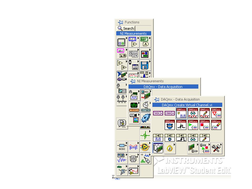
44 DAQmx Create Virtual Channel.vi
• Analog Input • Analog Output • Digital Input Digital Output • Counter Input Counter Ouput

45 DAQmx Create Virtual Channel.vi
NI-DAQmx Create Virtual Channel function possui diferentes possibilidades correspondentes ao tipo específico de medida ou geração de desempenho de canal virtual.

46 physical channels (analog input and analog output),
As entradas da NI-DAQmx Create Virtual Channel function diferem para cada exemplo. Entretanto certas entradas são comuns para todas. Por exemplo, entrada é exigida especificar se serão usados: physical channels (analog input and analog output), lines (digital), ou counter that the virtual channel(s) Analog input, analog output e counter utilizam minimum value e maximum value

47 Adquirir uma Amostra

48 Adquirir uma Amostra

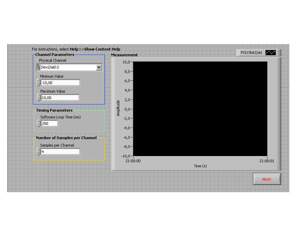
49 Adquirir uma Amostra – Painel Frontal

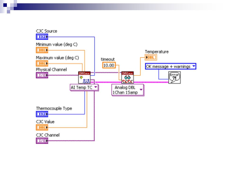
50 Fazer vi para adquirir sinal de um termopar

51 termocouple.vi

52 termocouple.vi

53 Adquirir sinal de múltiplos canais

54

55 NI-DAQmx: Reduce Development Time and Improve Performance

56 10 Funções no NI-DAQmx

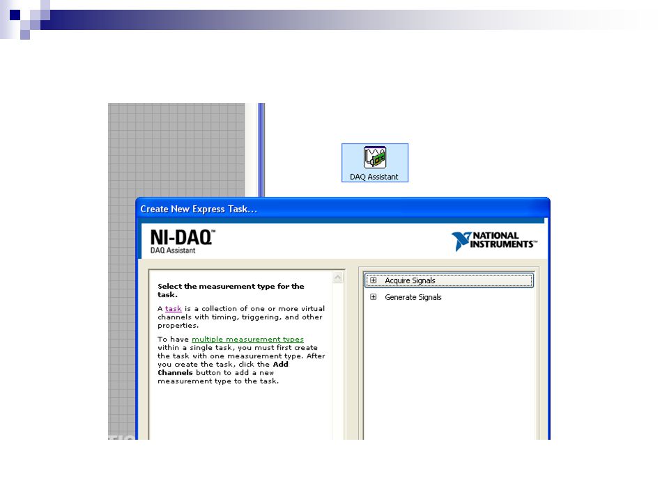
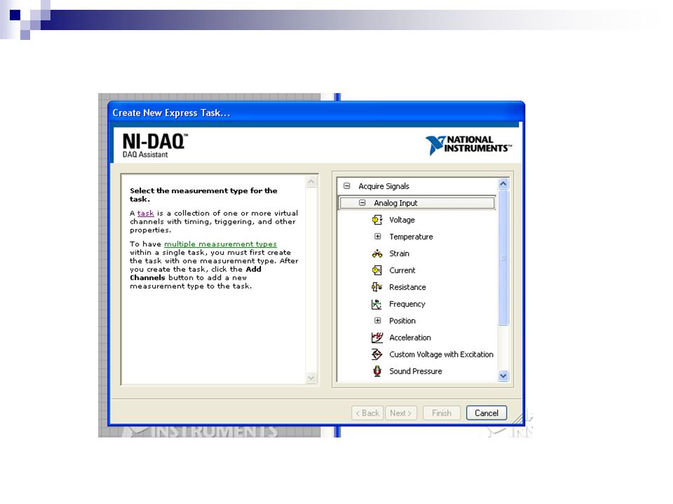
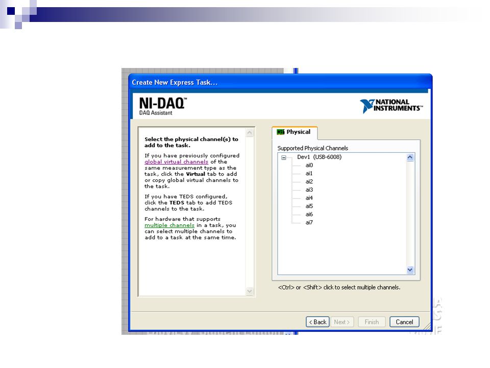
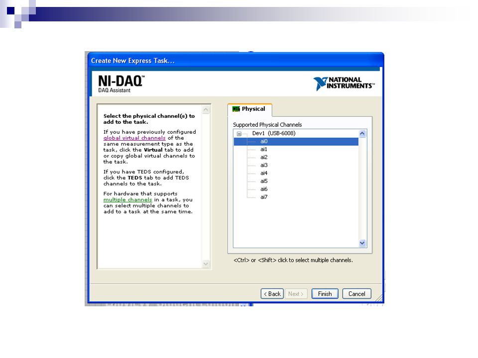
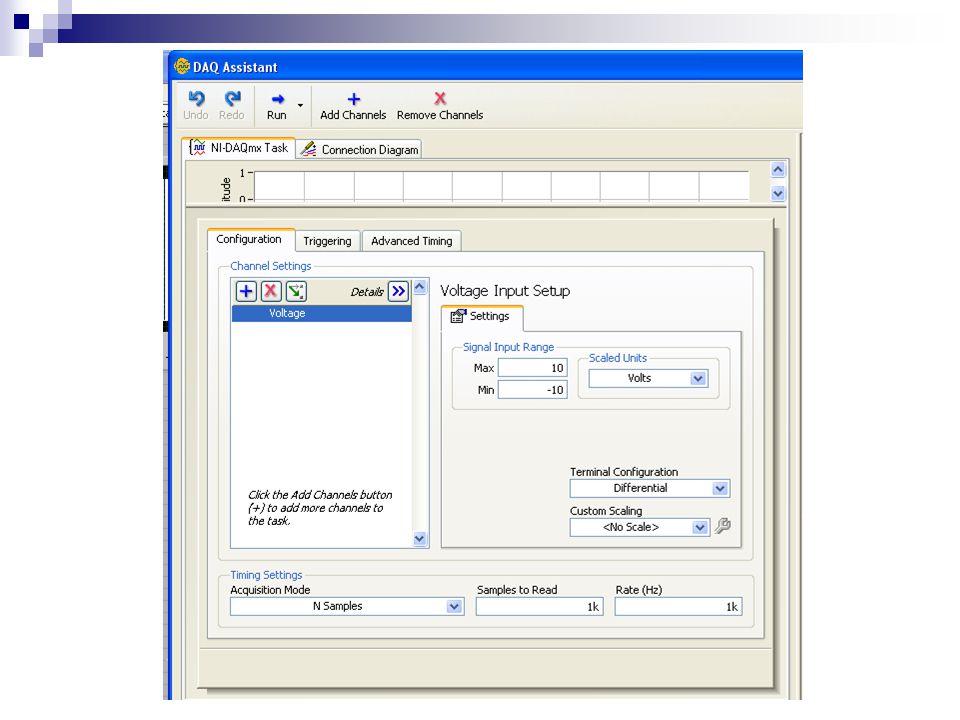
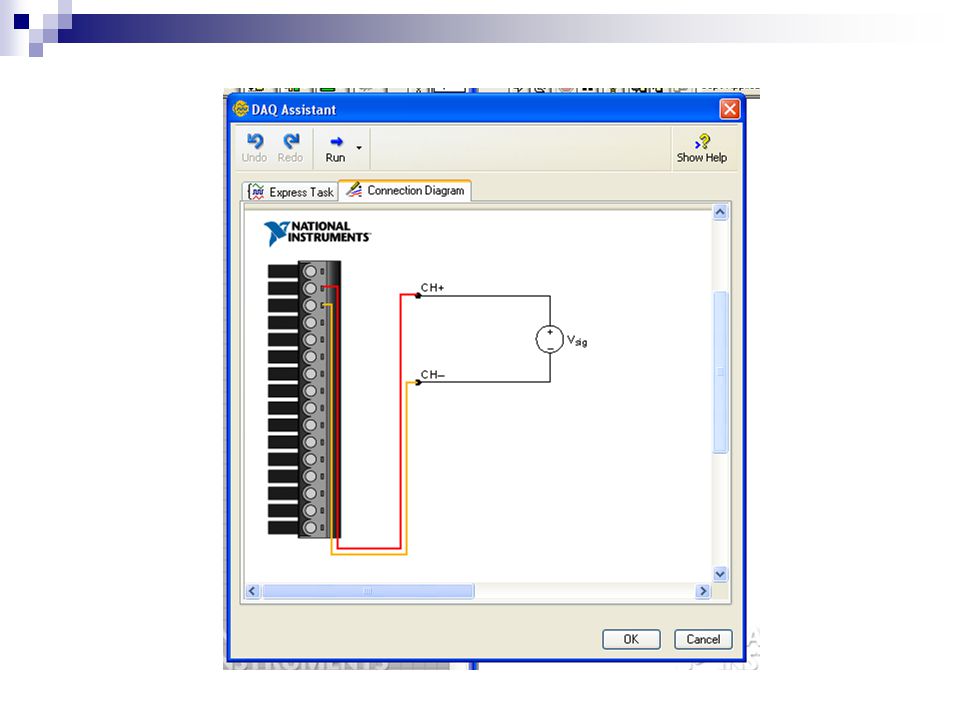
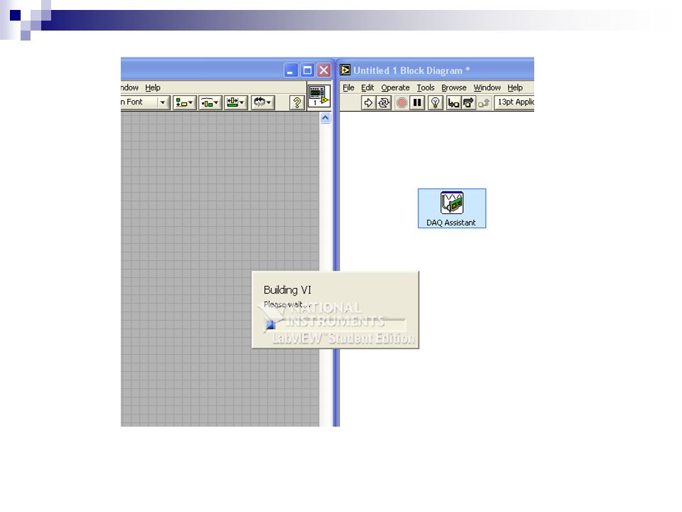
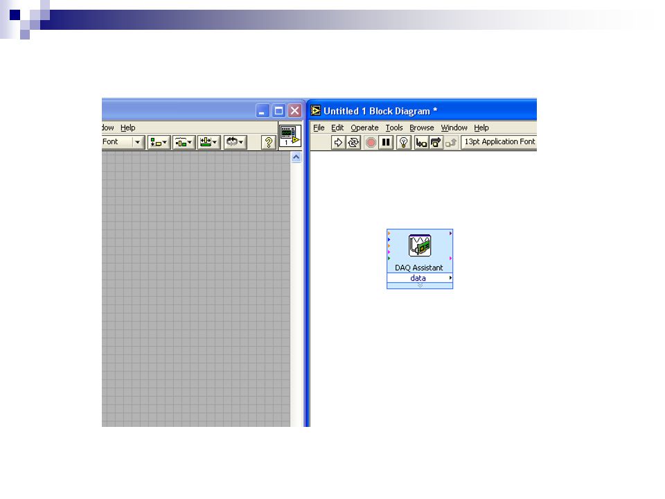
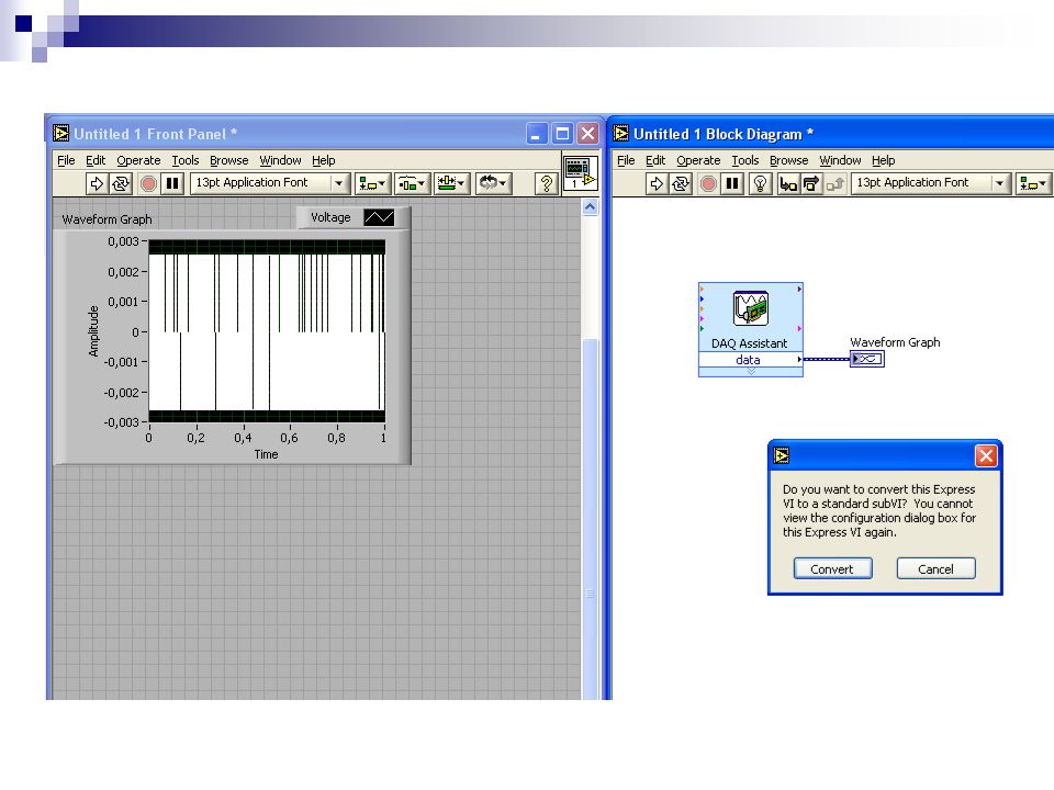
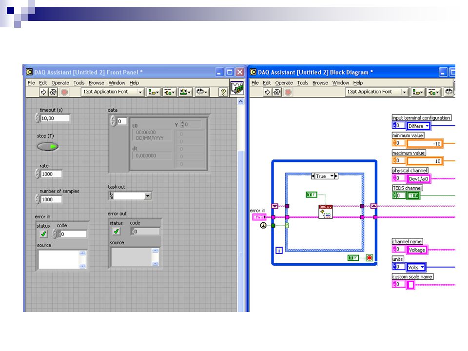
57 DAQ Assistant

58 DAQ Assistant DAQ Assistant é uma interface gráfica para iterativamente criar, editar e rodar NI-DAQmx virtual channels and tasks. NI-DAQmx virtual channel consiste de canais físicos em um dispositivo DAQ e informações de configuração para este canal físico, tal como range de entrada e escala. NI-DAQmx task é uma coleção de canais virtuais, timing e informação de triggering e outras propriedades referentes a aquisição ou geração. DAQ Assistant será configurado para medidas de estiramento.

59

60

61

62

63

64

65

66

67

68

69

70

71

72 DAQmx Trigger.vi

73 The NI-DAQmx Trigger function configura um disparo (trigger) para desempenhar uma ação específica. As mais comuns são start trigger e um reference trigger. Start trigger inicia uma aquisição ou geração. Reference trigger estabelece a posição em uma série de amostras adquiridas, onde dados pretrigados finalizam e dados pós-trigados inicializam. Ambos podem ser configurados para ocorrer em um digital edge, um analog edge, ou quando um sinal analógico entra ou sai de uma janela. No diagrama de blocos, tato o start quanto a reference são configurados utilizandoNI-DAQmx Trigger VI para ocorrer no digital edges para uma entrada analógica.

74

75 Visão arranjo de dados

76 A principal diferença entre Analog Input, AI Sample Channel em relação a Acquire Waveform é que esta ultima realiza medidas de uma forma de onda. Isto não é necessário em experimentos como termistor ou strain gage, uma vez que tais medidas não variam muito no tempo. Entretanto em experimentos com oscilações tempo é variável importantíssima. Também em experimentos onde tempo não é importante são necessárias menores taxas de aquisição. Acquire Waveform Sub VI amostra no tempo é feita por hardware localizados na placa de aquisição. Dados amostragem de tensão são estocados na memória usando acesso direto de memória (DMA). A amostragem pode ser realizada em altas taxas de amostragem, acima de 100,000 samples por segundo. Se dois canais estão sendo amostrados, cada canal terá 50,000 samples por segundo. Comparando, quando aquisição e estocagem são controladas por software, como com Sample Channel Sub VI, a máxima taxa de de aproximadamente 100 samples por segundo.

77 Adquirir dados e ler dados provenientes do buffer da placa de aquisição são duas operações separadas. Valores Default são utilizados para otimizar a aplicação. Passos de partida e leitura usam valores default -1 para number of scans to acquire e number of scans to read, respectivamente, o buffer size ajusta o número de scan para ambos os passos. Após aquisição buffer size scans, a aquisição está completa. Um passo limpa e libera o buffer da memória e outros rescursos são utilizados. A taskID “cadeia” VIs junta para controlar a ordem de execução (data dependency). Erros são passados de uma VI para outra através error in e error out clusters. Simple Error Handler VI no fim da sequência relatam informações quando ocorre um erro.

78 Buffer?? Um buffer é uma região da memória usada para reter temporariamente dados de entrada ou saída. Os dados de entrada ou saída podem ser provenientes de dispositivos fora do computador ou processos internos. Buffers podem ser implementados em hardware ou por software, a vasta maioria são implementadas por software. Buffers são utilizados quando existe diferença entre a taxa na qual os dados são recebidos e a taxa na qual são processados, ou quando tais taxas são variáveis, por exemplo em uma impressora.

79 Buffer (cont) Buffer – é como uma cesta para estocar doces ‘’temporariamente’’.

80 Analog Input Operations
Sequência AI Config -- Configura canais, ganhos e buffer do computador AI Start Seta condições de disparo, clocks de programa, e partida da DAQ AI Read Lê dados do buffer (repete se contínuo) AI Clear------Pára a DAQ, placa e recursos do micro livres Parâmetros Gerais VI taskID – para controlar ordem de execução Terminais Negrito Valores Default Pages 9-46 to 9-48: Discuss the standard sequence of the analog input operations. Explain how each sequence step translates to an intermediate Analog Input VI. Each of these VIs has several inputs and outputs. Show the help window information for each VI and discuss the important connections they will need to make such as taskID, required inputs, and error in/error out.

81 Analog Input Intermediate VIs
Buffered Analog Input Pages 9-49 to 9-50: Explain the nonbuffered application algorithm. Now explain the buffered application algorithm. Discuss the following points: Acquiring the data and reading the data from the DAQ board’s buffer are two separate operations. Default values are used to optimize the application. Because the start and read steps use the default value of -1 for number of scans to acquire and number of scans to read, respectively, the buffer size sets the number of scans for both steps. After acquiring buffer size scans, the acquisition is complete. The clear step frees the buffer memory and other resources used. The taskID “chains” the different VIs together to control the order of execution. Error information is passed from one VI to the next through the error in and error out clusters. The Simple Error Handler VI at the end of the sequence reports information on the first error that occurred, if any. Now explain how the continuous buffered acquisition works by simply setting the board to acquire continuously and then reading the buffer in a While Loop. Continuous Data Acquisition

82 Observação Dados estocados enquanto lê ou escreve, reduz o número de acesso exigido na fonte. Fluxos estocados (buffer) são mais eficientes do que similares non-buffred.

83 Analog Input Intermediate VIs
Buffered Analog Input Pages 9-49 to 9-50: Explain both nonbuffered and buffered operation. Discuss the following points: Acquiring the data and reading the data from the DAQ board’s buffer are two separate operations. Default values are used to optimize the application. Because the start and read steps use the default value of -1 for number of scans to acquire and number of scans to read, respectively, the buffer size sets the number of scans for both steps. After acquiring buffer size scans, the acquisition is complete. The clear step frees the buffer memory and other resources used. The taskID “chains” the different VIs together to control the order of execution (data dependency). Error information is passed from one VI to the next through the error in and error out clusters. The Simple Error Handler VI at the end of the sequence reports information on the first error that occurred, if any. Now explain how the continuous buffered acquisition works by simply setting the board to acquire continuously and then reading the buffer in a While Loop. Continuous Data Acquisition