Visão estéreo - correspondência e reconstrução -

Apresentação em tema: "Visão estéreo - correspondência e reconstrução -"— Transcrição da apresentação:

1 Visão estéreo - correspondência e reconstrução -
Cap. 7 Trucco & Verry

2 Reconstrução da forma

3 Captura de movimento

4 Basic principle to recover position from stereo images: Triangulation
Requires correspondence and camera calibration

5 Correpondência por semelhança
Sum of Square Differences – SSD ou Correlação

6 Correspondência por vizinhança correlacionada

7 Semelhança de duas regiões WW (SSD – Sum of Squared Difference)
x0+u y0+v y0 x0

8 Semelhança de duas regiões WW (correlação)
constante constante

9 Semelhança de duas regiões WW (Normalização)
Normalizando:

10 Correspondence between points
With characteristics - 

11 Correspondence problems: Oclusion
- 

12 Correspondence problem: lack of characterists
-  Ostridge egg on a Chinese checker board 

13 Correspondência com luz estruturada
Estéreo Ativo

14 Taxonomy of active range acquisition methods
Transmissive Sonar Non-contact Non-optical Microwave radar Reflective Shape from focus Shape from shading Active shape acquisition Passive Shape from silhouettes Slices … Destructive Optical Radar Contact Active Triangulation Non destructive Active depth from defocus Active stereo CMM … Asla Sá et al, Coded Structure Light for 3D-Photograpy: an Overview, Revista de Informática Teórica e Aplicada, Volume IX, Número 2, Porto Alegre, 2002 Brian Curless. New Methods for Surface Reconstruction from Range Images. PhD Dissertation. Stanford University. 1997

15 Active stereo solution
Use a light source to mark corresponding points uncalibrated light source calibrated light source One point at the time: long capture process. 

16 Active stereo: capturing many points
Use of a digital projector as a structured light source Pattern with several elements in a way where each element can be identified univocally point coding: prone to errors stripes: more robust

17 Methods for light coding: temporal codification
Project, in sequence, a series of slides that code in the image a binary number. n slides for 2n stripes. Two ilumination levels. Static scene. Code one axis. can be also 111 or 001! slide1 slide2 slide3 code problem: all transitions occur in the same place! Posdamer, J. L. Altschuler, M. D. Surface Measurement by Space-Encoded Projected Beam Systems. Comput. Graphics Image Process. 18, pp. 1-17, 1982.

18 Código de Gray  código binário
1 bit: 2 bits: 3 bits: Código de Gray 2 bits: 3 bits: ordem invertida

19 Código de Gray  código binário
Código binário Código de Gray

20 Robust temporal codification: Gray coding
transitions occur in different places Inokuchi, Seiji. Sato, Kosuki. Matsuda, Fumio. Range Imaging for 3D Object Recognition. Proc. Int. Conf. on Pattern Recognition, pp , 1984.

21 Example of Gray coding needs too many slides! 

22 Color Gray coding  reduces the number of slides by 3 better yet…

23 (b,s)-BCSL Coding 20 Sá, Asla Medeiros. Medeiros, Esdras Soares. Carvalho, Paulo Cezar Pinto. Velho, Luiz. Coded Structured Light for 3D-Photography: an Overview. Revista de Informática Teórica e Aplicada, Vol. 9, No. 2, outubro 2002

24 A practical difficulty in the border detection
example with the monochrome Gray code

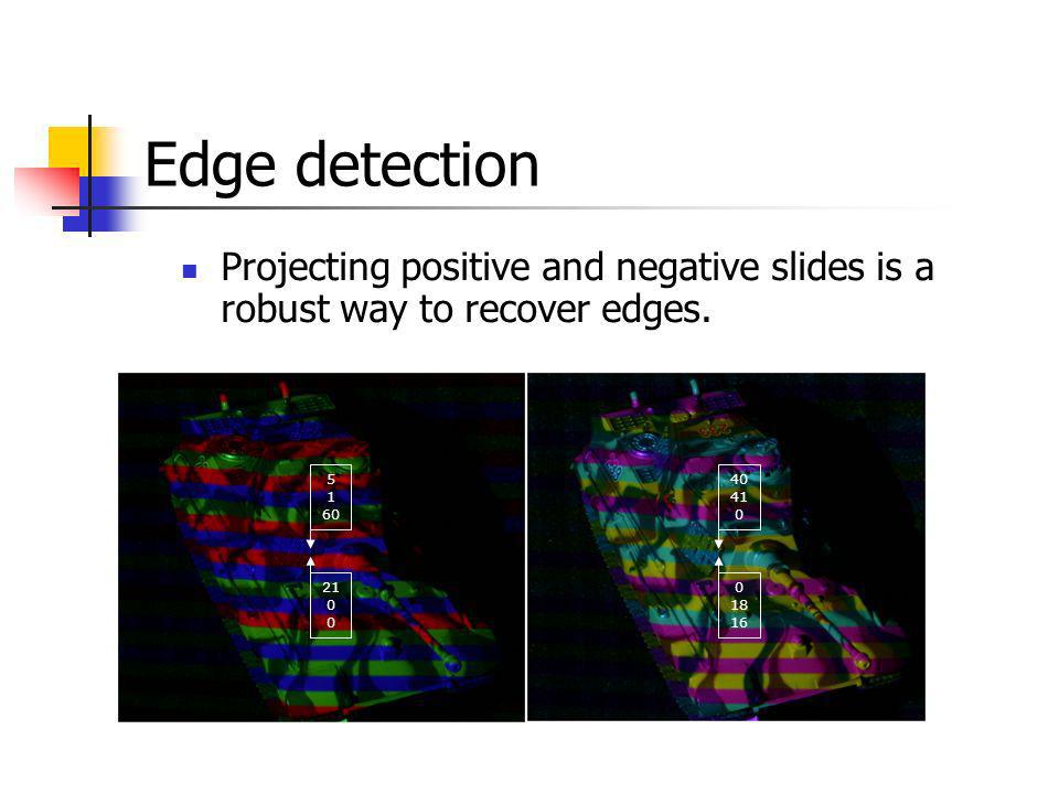
25 Edge detection Projecting positive and negative slides is a robust way to recover edges. 5 1 60 40 41 21 18 16

26 32rgb-BCSL coding (+) (-) slide 1 slide 2

27 Recovering colored codes
ambient light reflection factors projected light  negative slide  positive slide

28 Implementação do BCSL //A função getBcslStripeCode retorna o código de transição de faixa conforme a seqüência de cores fornecida. //Observe a ordem em que as cores devem ser passadas: // Primeiro as cores da imagem 1 e depois da imagem 2 // Primeiro a faixa da esquerda e depois a faixa da direita // //O código das cores e das bases é conforme a tabela abaixo. //Padrão 3_2 //base 3 //1 - vermelho //2 - verde //3 - azul //Padrão 4_2 //base 4 //4 - magenta //Padrão 6_2 //base 6 //4 - ciano //5 - magenta //6 - amarelo int getBcslStripeCode(int base, int colorLeft1, int colorRight1,int colorLeft2, int colorRight2);

29 teoria pode ser complicada mas a implementação é muito simples!
int matrix3_2[4*9]={ 0, 3, 6, 9, 14, 17, 19, 11, 28, 34, 22, 24, 26, 29, 18, 21, 1, 31, 33, 35, 15, 4, , 13, 16, , , 12, 27, 5, , 25, 2, , 20, 30 }; …. int getBcslStripeCode(int base, int colorLeft1, int colorRight1,int colorLeft2, int colorRight2) { int aux1, aux2,linha,coluna; colorLeft2--; colorRight2--; colorLeft1--; colorRight1--; linha = (colorLeft1 * base) + colorLeft2; aux1 = (colorRight2 - colorLeft2); aux2 = (colorRight1 - colorLeft1); aux1 = (aux1>0)?(aux1-1):((base-1)+aux1); aux2 = (aux2>0)?(aux2-1):((base-1)+aux2); coluna = ((aux2) * (base-1)) + (aux1); switch(base){ case 3: return matrix3_2[linha *4+coluna]; break; case 4: return matrix4_2[linha *9 +coluna]; case 6: return matrix6_2[linha *25 +coluna]; default: printf("Error: invalid BCSL base\n"); return -1; } teoria pode ser complicada mas a implementação é muito simples!

30 Disparidade x Profundidade
Mapa de profundiade Disparidade x Profundidade

31 Disparidade

32 Profundidade versus disparidade
Z xl xr cl cr f ol or x x z z T

33 Correspondência pela Geometria das Câmeras
Geometria Epipolar Correspondência pela Geometria das Câmeras

34 Epipolar Geometry ctd. Guido Gerig

35 Geometria Epipolar: notação
Pl pl Linha epipolar pr Pr ycl xcr ycr zcr xcl el er Or Ol zcl

36 Example: converging cameras

37 Example: motion parallel with image plane

38 Example: forward motion

39 Geometria Epipolar: relações básicas
xcl ycl zcl xcr ycr zcr

40 Produto vetorial (revistado)

41 Matriz Essencial Pl Pr P Matriz essencial ycr xcr zcr ycl xcl er el
eye l P eye r Pl pl xcl ycl zcl xcr ycr zcr pr Pr el er Matriz essencial

42 Parâmetros extrínsecos
xc yc zc Pc t yw xw zw Pw

43 Rotação de a para b (left to right)

44 Vetor do eye de b em a ycl xcl eye l Z w zcl ycr Y w xcr eye r zcr X w

45 Glu Look At void gluLookAt(GLdouble eyex, GLdouble eyey, GLdouble eyez, GLdouble centerx, GLdouble centery, GLdouble centerz, GLdouble upx, GLdouble upy, GLdouble upz); Dados: eye, center, up (definem o sistema de coordenadas do olho) Determine a matriz que leva do sistema de Coordenadas dos Objetos para o sistema de Coordenadas do Olho up eye center Coordenadas dos objetos Coordenadas do olho eye

46 Calculo do sistema - xe ye ze
center eye zo yo xo ze xe up dados: eye, center, up

47 Translada o eye para origem
center eye zo yo xo ze xe ye zo yo xo center eye ze xe ye

48 Roda xe ye ze para xw yw zw
zo yo xo center eye ze xe ye xe , xo ye , yo ze , zo

49 Matriz LookAt do OpenGL

50 Matriz essencial (código C)
Matrix epiEssencialMatrix( Matrix Ra, Vector eye_a, Matrix Rb, Vector eye_b) { Matrix Rba = algMult(Rb,algTransp(Ra)); Vector eye = algMult(Ra,algSub(eye_b,eye_a); Matrix S = algVectorProductMatrix(eye); Matrix E = algMult(Rba,S); return E; }

51 Matriz Essencial P Pl Pr pl pr xcl ycl zcl xcr ycr zcr el er Ol T Or

52 Câmera para imagem

53 Geometria Epipolar: Matriz Fundamental

54 Matriz fundamental Pode ser estimada diretamente se conhecermos pelo menos oito pares de pontos correspondentes

55 Transformações do OpenGL
center eye zo yo xo up xe ye ze xn yn zn

56 Matriz de projeção ye ze xe ye ze xe 8 4 7 3 5 1 2 6 [ H ] = ? 8 4 3 7

57 Transforma o prisma de visão cubo normalizado [-1,1]×[-1,1] ×[-1,1]
xe ye ze -(r-l)/2 (r-l)/2 -(t-b)/2 (t-b)/2 (f-n)/2 -(f-n)/2 xe ye ze l r b t xn yn zn 1 -1 near far xe ye ze 1 -1 far near

58 Matriz Frustum do OpenGL
OpenGL Spec

59 Transformação para o viewport
void glViewport(int x0, int y0, int w, int h ); xw yw w h y0 x0 xn yn zn 1 -1 zw[0.. zmax], zmax = 2n-1 geralmente 65535

60 Revendo as transformações

61 Sistemas de coordenadas
yim yc y' eixo óptico zc y0 x' oc xc x0 pixel f xim yim sy y' sx vista lateral yc oy fovy zc h sy x' oc ox xim f =n w sx

62 Revendo as transformações

63 Matriz Fundamental (código C)
Matrix epiFundamentalMatrix( Matrix Ma, Matrix Ra, Vector eye_a, Matrix Mb, Matrix Rb, Vector eye_b) { Matrix E = epiEssencialMatrix(Ra,eye_a,Rb,eye_b); Matrix invMa = algInv(Ma); Matrix invMbTransp = algTransp(algInv(Mb)); Matrix tmp = algMult(invMbTransp,E); Matrix F = algMult(tmp,invMa); return F; }

64 Estimativa direta da Matriz Fundamental
O algoritmo de 8 pontos

65 Estimating Fundamental Matrix
The 8-point algorithm Each point correspondence can be expressed as a linear equation

66 Estimating Fundamental Matrix
The 8-point algorithm F é a coluna de V correspondente ao menor valor singular

67 Estimating Fundamental Matrix
The 8-point algorithm deveria ter posto 2! Seja D' = D com o menor valor singular = 0

68 The Normalized 8-point Algorithm
Richard Hartley

69 The Normalized 8-point Algorithm
Richard Hartley centróide escale para a distância média ficar em

70 Retificação de Imagens

71 Retificação UNC-CH

72 Rectification ctd. before after Guido Gerig

73 Retificação de imagens
Trucco e Verri y' yc z' zc O O' x' xc ponto principal

74 Retificação de imagens
Trucco e Verri P ycl pl xcr ycr zcr pr xcl el T er Or Ol zcl

75 Retificação de imagens
Trucco e Verri 1. Construa: Pr= R(Pl - T) 2. Defina: 3. Aplique: 3. Aplique:

76 Stereo image rectification
Steve Seitz, University of Washington

77 Stereo image rectification
Image Reprojection reproject image planes onto common plane parallel to line between optical centers a homography (3x3 transform) applied to both input images pixel motion is horizontal after this transformation C. Loop and Z. Zhang. Computing Rectifying Homographies for Stereo Vision. IEEE Conf. Computer Vision and Pattern Recognition, 1999. Steve Seitz, University of Washington

78 Image Rectification Common Image Plane Parallel Epipolar Lines
Search Correspondences on scan line Steve Seitz, University of Washington

79 Reconstrução

80 Reconstrução por triangulação

81 Reconstrução por triangulação

82 Outro processo de reconstrução
Miguel Ribo, Axel Pinz, Anton L. Fuhrmann “A new Optical Tracking System for Virtual and Augmented Reality Applications”,

83 Reconstruction O O’ p p’ Steve Seitz, University of Washington

84 Reconstruction Equation 1 Equation 2 (From equations 1 and 2)
Steve Seitz, University of Washington

85 Reconstruction up to a Scale Factor
Assume that intrinsic parameters of both cameras are known Essential Matrix is known up to a scale factor (for example, estimated from the 8 point algorithm). Steve Seitz, University of Washington

86 Reconstruction up to a Scale Factor
Steve Seitz, University of Washington

87 Reconstruction up to a Scale Factor
Let It can be proved that Steve Seitz, University of Washington

88 Reconstruction up to a Scale Factor
We have two choices of t, (t+ and t-) because of sign ambiguity and two choices of E, (E+ and E-). This gives us four pairs of translation vectors and rotation matrices. Steve Seitz, University of Washington

89 Reconstruction up to a Scale Factor
Given and Construct the vectors w, and compute R Reconstruct the Z and Z’ for each point If the signs of Z and Z’ of the reconstructed points are both negative for some point, change the sign of and go to step 2. different for some point, change the sign of each entry of and go to step 1. both positive for all points, exit. Steve Seitz, University of Washington

90 Proposed system: equipament
2 cameras and 1 projector (fast) 1 moving camera and 1 projector (slow)

91 Proposed system: 32rgb-BCSL coding
positive slide positive slide negative slide left right

92 Where is a point in the other image?
u u

93 One solution: (u,v) coordinates
double the number of photos!

94 Epipolar geometry P Pl Epipolar Pr Line pl ycr ycl pr xcr xcl er el
zcr xcl el er eyer eyel zcl

95 Epipolar correspondence

96 Reconstruction by triangulation: ideia

97 Reconstruction by triangulation: algebra

98 Captured data

99 Cylinder model covariance matrix: centroid: axis of the points pi:

100 Initial cylinder adjustment
tangent plane perpendicular to ê3: first guess for cc: first guess for zc:

101 Results of the initial cylinder adjustment

102 Model fitting problem Giving a set of points P and a model Q, find the rigid body motion (R, t) that minimizes: where q(pi) is the point in Q correspondent to pi.

103 ICP (Iteractive Closest Point) Algorithm
begins with a initial guess for the model pose( R and t ) at each iteration, q(pi) is the point in Q closest to Rpi + t R e t are computed to minimize the error P. J. Besl and N. D. McKay, A Method for Registration of 3-D Shapes, IEEE Transactions on Pattern Analysis and Machine Intelligence, Vol. 14, No. 12, February 1992

104 Projection of a point on a cylinder
Given : Plane : Compute : Axis : 

105 ICP step find centroids: p0 e q0 Define pi’= pi – p0 , qi’= qi – q0
where Rotation: R = M(MT M) –1/2 Translation: t = q0– Rp0

106 Results

107 Direct measure