Visão estéreo - correspondência e reconstrução -.

Apresentação em tema: "Visão estéreo - correspondência e reconstrução -."— Transcrição da apresentação:

1 Visão estéreo - correspondência e reconstrução -

2 Reconstrução da forma

3 Captura de movimento

4 Basic principle to recover position from stereo images: Triangulation Requires correspondence and camera calibration

5 Mapa de profundiade Disparidade x Profundidade

6 Profundidade versus disparidade z x olol x oror z P clcl crcr xlxl xrxr T Z f

7 Uso do mapa de profundidade Cesar Palomo Larry Zitnick

8 Time slice, bullet-time or frozen time effects

9 Correpondência por semelhança Sum of Square Differences – SSD ou Correlação

10 Correspondência por vizinhança correlacionada

11 Semelhança de duas regiões W  W (SSD – Sum of Squared Difference) x0x0 y0y0 x0+ux0+u y0+vy0+v

12 Semelhança de duas regiões W  W (correlação) constante  constante

13 Semelhança de duas regiões W  W (Normalização) Normalizando:

14 Correspondence between points With characteristics  -

15 Correspondence problems: Oclusion  -

16 Correspondence problem: lack of characterists  - Ostridge egg on a Chinese checker board

17

18 Correspondência com luz estruturada Estéreo Ativo

19 Taxonomy of active range acquisition methods Active shape acquisition Contact Non destructive Non-contact Transmissive Reflective CT Asla Sá et al, Coded Structure Light for 3D-Photograpy: an Overview, Revista de Informática Teórica e Aplicada, Volume IX, Número 2, Porto Alegre, 2002 Brian Curless. New Methods for Surface Reconstruction from Range Images. PhD Dissertation. Stanford University. 1997 Non-optical Sonar Microwave radar Optical Radar Triangulation Active stereo Active depth from defocus Passive Shape from focus Destructive Slices CMM Shape from shading Shape from silhouettes Active … …

20 Active stereo solution Use a light source to mark corresponding points uncalibrated light sourcecalibrated light source One point at the time: long capture process. 

21 Active stereo: capturing many points Use of a digital projector as a structured light source Pattern with several elements in a way where each element can be identified univocally point coding: prone to errorsstripes: more robust

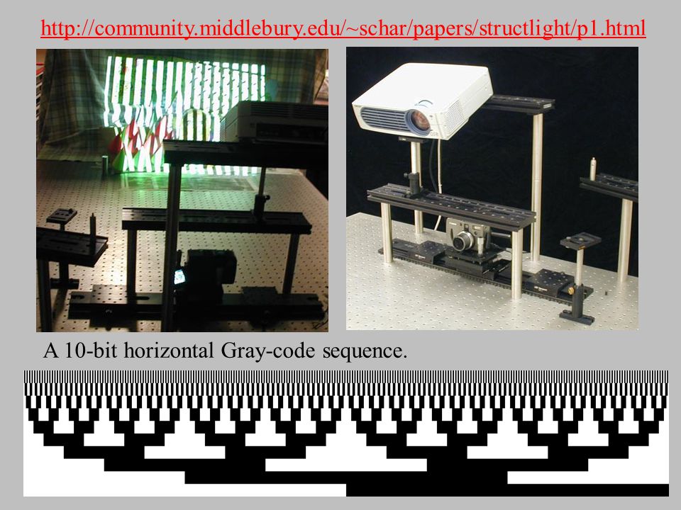
22 Methods for light coding: temporal codification Project, in sequence, a series of slides that code in the image a binary number. n slides for 2 n stripes. Two ilumination levels. Static scene. Code one axis. Posdamer, J. L. Altschuler, M. D. Surface Measurement by Space-Encoded Projected Beam Systems. Comput. Graphics Image Process. 18, pp. 1-17, 1982. slide1slide2codeslide3 problem: all transitions occur in the same place! can be also 111 or 001!

23 Código de Gray  código binário Código binário 1 bit: 0 1 2 bits: 00 01 10 11 3 bits:000001010011100101110111 Código de Gray 1 bit: 0 1 2 bits: 00 01 11 10 3 bits:000001011010110111101100 ordem invertida

24 Código de Gray  código binário Código binárioCódigo de Gray

25 Robust temporal codification: Gray coding Inokuchi, Seiji. Sato, Kosuki. Matsuda, Fumio. Range Imaging for 3D Object Recognition. Proc. Int. Conf. on Pattern Recognition, pp.806-808, 1984. transitions occur in different places

26 Example of Gray coding needs too many slides! 

27 A 10-bit horizontal Gray-code sequence. http://community.middlebury.edu/~schar/papers/structlight/p1.html

28 Color Gray coding better yet… reduces the number of slides by 3 

29 (b,s)-BCSL Coding Sá, Asla Medeiros. Medeiros, Esdras Soares. Carvalho, Paulo Cezar Pinto. Velho, Luiz. Coded Structured Light for 3D-Photography: an Overview. Revista de Informática Teórica e Aplicada, Vol. 9, No. 2, outubro 2002 20

30 A practical difficulty in the border detection example with the monochrome Gray code

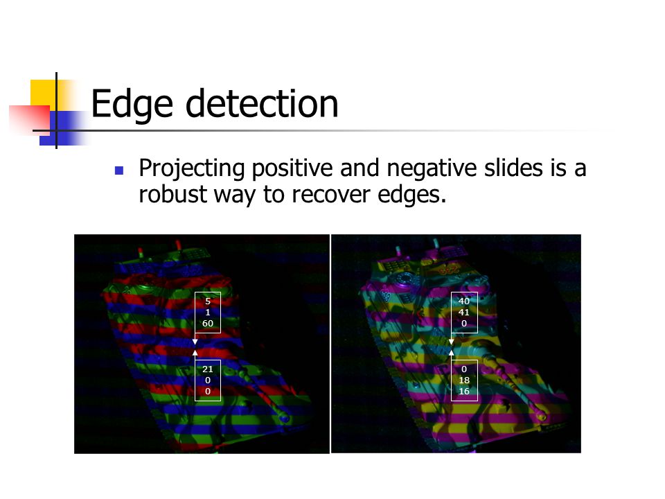
31 Edge detection Projecting positive and negative slides is a robust way to recover edges. 5 1 60 21 0 40 41 0 18 16

32 32rgb-BCSL coding (+) (-) slide 1slide 2

33 Recovering colored codes  negative slide  positive slide ambient light reflection factors projected light

34 Implementação do BCSL //A função getBcslStripeCode retorna o código de transição de faixa conforme a seqüência de cores fornecida. //Observe a ordem em que as cores devem ser passadas: //Primeiro as cores da imagem 1 e depois da imagem 2 //Primeiro a faixa da esquerda e depois a faixa da direita // //O código das cores e das bases é conforme a tabela abaixo. //Padrão 3_2 //base 3 //1 - vermelho //2 - verde //3 - azul //Padrão 4_2 //base 4 //1 - vermelho //2 - verde //3 - azul //4 - magenta //Padrão 6_2 //base 6 //1 - vermelho //2 - verde //3 - azul //4 - ciano //5 - magenta //6 - amarelo int getBcslStripeCode(int base, int colorLeft1, int colorRight1,int colorLeft2, int colorRight2);

35 int getBcslStripeCode(int base, int colorLeft1, int colorRight1,int colorLeft2, int colorRight2) { int aux1, aux2,linha,coluna; colorLeft2--; colorRight2--; colorLeft1--; colorRight1--; linha = (colorLeft1 * base) + colorLeft2; aux1 = (colorRight2 - colorLeft2); aux2 = (colorRight1 - colorLeft1); aux1 = (aux1>0)?(aux1-1):((base-1)+aux1); aux2 = (aux2>0)?(aux2-1):((base-1)+aux2); coluna = ((aux2) * (base-1)) + (aux1); switch(base){ case 3: return matrix3_2[linha *4+coluna]; break; case 4: return matrix4_2[linha *9 +coluna]; break; case 6: return matrix6_2[linha *25 +coluna]; break; default: printf("Error: invalid BCSL base\n"); return -1; } int matrix3_2[4*9]={ 0, 3, 6, 9, 14,17,19,11, 28,34,22,24, 26,29,18,21, 1,31,33,35, 15, 4, 8,13, 16, 23, 32,12, 27, 5, 7,25, 2, 10,20,30 }; …. teoria pode ser complicada mas a implementação é muito simples!

36 Geometria Epipolar Correspondência pela Geometria das Câmeras

37 Guido Gerig Epipolar Geometry ctd.

38 Geometria Epipolar: notação OlOl P OrOr PlPl plpl x cl y cl z cl x cr y cr z cr prpr PrPr elel erer Linha epipolar Linha epipolar

39 Example: converging cameras

40 Example: motion parallel with image plane

41 Example: forward motion e e’

42 Geometria Epipolar: relações básicas P x cl y cl z cl x cr y cr z cr

43 MGattass Produto Vetorial forma de lembrar

44 MGattass Matriz do produto vetorial

45 Produto misto (revistado) h

46 Matriz Essencial Matriz essencial eye l P eye r PlPl plpl x cl y cl z cl x cr y cr z cr prpr PrPr elel erer

47 Rotação de a para b (left to right)

48 Vetor do eye de b em a X w Y w Z w eye l x cl y cl z cl x cr y cr z cr eye r

49 Matriz essencial (código C) Matrix epiEssencialMatrix( Matrix Ra, Vector eye_a, Matrix Rb, Vector eye_b) { Matrix Rba = algMult(Rb,algTransp(Ra)); Vector eye = algMult(Ra,algSub(eye_b,eye_a); Matrix S = algVectorProductMatrix(eye); Matrix E = algMult(Rba,S); return E; }

50 Matriz Essencial T OlOl P OrOr PlPl plpl x cl y cl z cl x cr y cr z cr prpr PrPr elel erer

51 Câmera para imagem

52 Geometria Epipolar: Matriz Fundamental Matriz fundamental

53 Pode ser estimada diretamente se conhecermos pelo menos oito pares de pontos correspondentes

54 Matriz Fundamental (código C) Matrix epiFundamentalMatrix( Matrix Ma, Matrix Ra, Vector eye_a, Matrix Mb, Matrix Rb, Vector eye_b) { Matrix E = epiEssencialMatrix(Ra,eye_a,Rb,eye_b); Matrix invMa = algInv(Ma); Matrix invMbTransp = algTransp(algInv(Mb)); Matrix tmp = algMult(invMbTransp,E); Matrix F = algMult(tmp,invMa); return F; }

55 Estimativa direta da Matriz Fundamental O algoritmo de 8 pontos

56 Estimating Fundamental Matrix Each point correspondence can be expressed as a linear equation The 8-point algorithm

57 Estimating Fundamental Matrix The 8-point algorithm F é a coluna de V correspondente ao menor valor singular

58 Estimating Fundamental Matrix The 8-point algorithm deveria ter posto 2! Seja D' = D com o menor valor singular = 0

59 The Normalized 8-point Algorithm Richard Hartley

60 The Normalized 8-point Algorithm Richard Hartley centro escale para a distância média ficar em

61 Retificação de Imagens

62 Retificação UNC-CH

63 Rectification ctd. before after Guido Gerig

64 Retificação de imagens z'z' xcxc ycyc zczc y' x' O O' ponto principal Trucco e Verri

65 Retificação de imagens OlOl P OrOr plpl x cl y cl z cl x cr y cr z cr prpr elel erer T Trucco e Verri

66 Retificação de imagens Trucco e Verri 1. Construa: 2. Defina: 3. Aplique: P r = R(P l - T) 3. Aplique:

67 Reconstrução

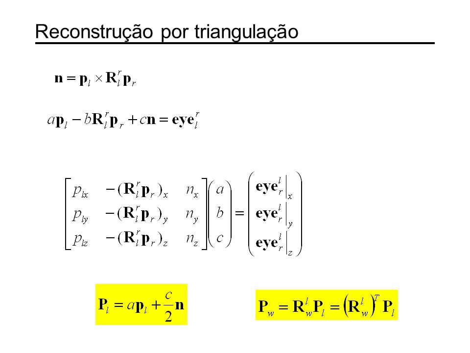
68 Reconstrução por triangulação

69

70 Outro processo de reconstrução Miguel Ribo, Axel Pinz, Anton L. Fuhrmann “A new Optical Tracking System for Virtual and Augmented Reality Applications”,

71 Reconstruction up to a Scale Factor Assume that intrinsic parameters of both cameras are known Essential Matrix is known up to a scale factor (for example, estimated from the 8 point algorithm). Steve Seitz, University of Washington

72 Reconstruction up to a Scale Factor Steve Seitz, University of Washington

73 Reconstruction up to a Scale Factor Let It can be proved that Steve Seitz, University of Washington

74 Reconstruction up to a Scale Factor We have two choices of t, (t + and t - ) because of sign ambiguity and two choices of E, (E + and E - ). This gives us four pairs of translation vectors and rotation matrices. Steve Seitz, University of Washington

75 Reconstruction up to a Scale Factor Given and 1.Construct the vectors w, and compute R 2.Reconstruct the Z and Z’ for each point 3.If the signs of Z and Z’ of the reconstructed points are a)both negative for some point, change the sign of and go to step 2. b)different for some point, change the sign of each entry of and go to step 1. c)both positive for all points, exit. Steve Seitz, University of Washington

76 Proposed system: equipament 2 cameras and 1 projector (fast) 1 moving camera and 1 projector (slow)

77 Proposed system: 32rgb-BCSL coding leftright positive slide negative slide

78 Where is a point in the other image? u u

79 One solution: (u,v) coordinates double the number of photos!

80 Epipolar geometry eye l P eye r PlPl plpl x cl y cl z cl x cr y cr z cr prpr PrPr elel erer Epipolar Line Epipolar Line

81 Epipolar correspondence

82 Reconstruction by triangulation: ideia

83 Reconstruction by triangulation: algebra

84 Captured data

85 Alinhamento de nuvens de pontos

86 Problema de alinhamento Dadas duas nuvens de pontos P e Q, encontrar o movimento rígido (R, t) que minimiza o erro de ajuste onde q(p i ) é o ponto em Q correspondente ao ponto p i de P. Dificuldade: não se sabe, a priori, qual é o ponto em Q que corresponde a p i

87 Algoritmo ICP (Iterative Closest Point) inicia com estimativa grosseira para R e t a cada iteração, q(p i ) é escolhido como o ponto em Q mais próximo de Rp i + t R e t são recalculados de modo a minimizar o erro de ajuste P. J. Besl and N. D. McKay, A Method for Registration of 3-D Shapes, IEEE Transactions on Pattern Analysis and Machine Intelligence, Vol. 14, No. 12, February 1992

88 Algoritmo ICP (Iterative Closest Point)

89 Também se aplica a ajuste de nuvens de pontos a modelos (por exemplo, cilindros)

90 Subproblema fundamental: alinhamento de pontos correspondentes Dados os pares de pontos correspondentes p i, q i (i = 1,..., n), determinar R e t que minimizam Resolvido por Horn[88, 89]

91 Alinhamento de pontos correspondentes –Obter os centróides p 0 e q 0 –Definir p i ’= p i – p 0, q i ’= q i – q 0 –Definir onde

92 Alinhamento de pontos correspondentes –Rotação: R = M(M T M) –1/2 –Translação: t = q 0 – Rp 0 –Observação: se a transformação é escrita na forma R(p + t), R não muda e t é simplesmente q 0 – p 0

93 Alinhamento de pontos correspondentes –Pode ser incluído um fator de escala: –Rotação: R = M(M T M) –1/2 –Escala: –Translação: t = q 0 – sRp 0

94 Exemplo (2D)

95 (  = 18 o )

96 Exemplo (2D)

97 Variantes do ICP ICP funciona melhor quando todo ponto em P corresponde a algum ponto em Q (não é o caso no alinhamento de malhas obtidas por fotografia 3D) Diversas estratégias para melhorar o desempenho para alinhamento de malhas com superposição parcial

98 Variantes do ICP Tomar pontos em ambas as malhas Usar outros critérios para casamento (textura, normal) Atribuir pesos às correspondências Rejeitar outliers Alterar a medida de distância (ponto- superfície no lugar de ponto-ponto)

99 Cylinder model axis of the points p i : covariance matrix: centroid:

100 Initial cylinder adjustment tangent plane perpendicular to ê 3 : first guess for c c : first guess for z c :

101 Results of the initial cylinder adjustment

102 Projection of a point on a cylinder Plane  :  Axis : Given : Compute :

103 Results

104 Direct measure

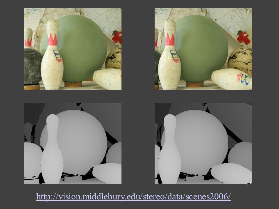
105 http://vision.middlebury.edu/stereo/data/scenes2006/