ENGA47 – TECNOLOGIA DOS MATERIAIS… Estrutura de Sólidos Cristalinos Prof. Dr. Vitaly F. Rodríguez-Esquerre.

Apresentação em tema: "ENGA47 – TECNOLOGIA DOS MATERIAIS… Estrutura de Sólidos Cristalinos Prof. Dr. Vitaly F. Rodríguez-Esquerre."— Transcrição da apresentação:

1 ENGA47 – TECNOLOGIA DOS MATERIAIS… Estrutura de Sólidos Cristalinos Prof. Dr. Vitaly F. Rodríguez-Esquerre

2 O que será estudado... Como os átomos se arranjam em estruturas sólidas? Como a densidade do material depende da sua estrutura? Estrutura cristalina dos sólidos

3 Os materiais sólidos podem ser classificados de acordo com a regularidade com a qual átomos e íons se arranjam em relação uns aos outros. Um material cristalino é aquele nos quais os átomos se repetem num arranjo periódico em largas distâncias atômicas. Todos os metais, muitos materiais cerâmicos e certos polímeros formam estruturas cristalinas sob condições normais de solidificação. ENGA47 – TECNOLOGIA DOS MATERIAIS…

4 As propriedades dos materials estão diretamente relacionadas às suas estruturas cristalinas. Por exemplo, cerâmicos e polímeros não cristalinos são em geral opticamente transparentes, ou seja permitem a passagem da luz, esses mesmos materiais na forma cristalina tendem a ser opacos, ou no melhor dos casos, translúcidos ENGA47 – TECNOLOGIA DOS MATERIAIS…

5 Os materiais que não possuem esta ordenação atômica a largas distâncias são chamados amorfos. Os vidros, por exemplo, não são cristalinos. A figura da esquerda apresenta um dos vidros mais simples (B2O3), no qual cada pequeno átomo de boro se aloja entre três átomos maiores de oxigênio. Como o boro é trivalente e o oxigênio bivalente, o balanceamento elétrico é mantido se cada átomo de oxigênio estiver entre dois átomos de boro. Como resultado, desenvolve-se uma estrutura contínua de átomos fortemente ligados. ENGA47 – TECNOLOGIA DOS MATERIAIS…

6 Não denso, empacotamento aleatório Denso, empacotamento ordenado Estruturas densas e com empacotamento ordenado tem Menores energias Energia e Empacotamento Energy r typical neighbor bond length typical neighbor bond energy Energy r typical neighbor bond length typical neighbor bond energy

7 átomos empacotados em arranjos 3D periódicos Materiais Cristalinos... -metais -muitos cerâmicos -alguns polímeros átomos não estão empacotados e não tem arranjo periodico Noncrystalline materials... - Estruturas complexas - Esfriamento rápido SiO 2 cristalino SiO 2 não cristalino "Amorfo" = Não Cristalino Materiais e Empacotamento SiOxygen típico de: acontece:

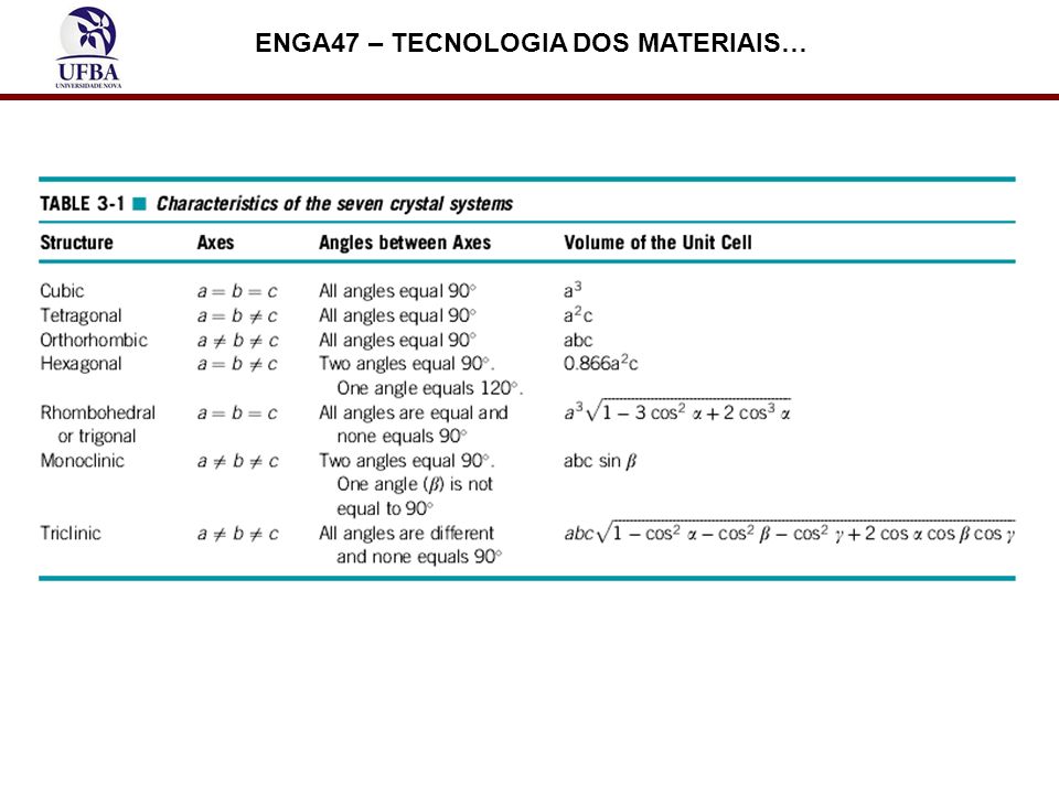
8 Sistemas Cristalinos 7 sistemas cristalinos 14 arranjos de cristais Célula unitária: menor volume repetitivo que contem o padrão completo do arranjo de um cristal. a, b, e c são as constantes periódicas

9 A maioria dos materiais de interesse para o engenheiro tem arranjos atômicos que se repetem nas três dimensões de uma unidade básica. Tais estruturas são denominadas cristais. Existem 7 tipos principais de cristais: cúbico, tetragonal, ortorrômbico, monoclínico, triclínico, hexagonal e romboédrico. Existem 14 redes de Bravais

10 (c) 2003 Brooks/Cole Publishing / Thomson Learning™ 14 Redes de Bravais

11 14 redes de Bravais agrupadas em 7 sistemas cristalinos ENGA47 – TECNOLOGIA DOS MATERIAIS…

12

13 Estruturas Metálicas Cristalinas Como pode-se arranjar átomos metálicos para minimizar o espaço vazío? 2-dimensões vs. Agora arranje estas camadas 2-D para fazer estruturas cristalinas 3-D ENGA47 – TECNOLOGIA DOS MATERIAIS…

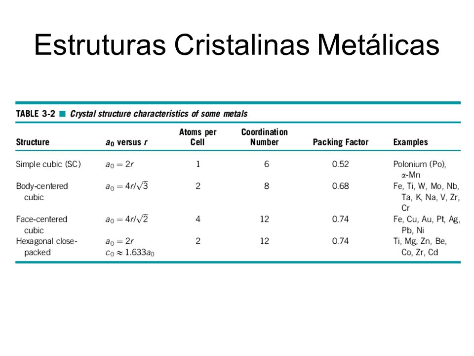
14 São densamente empacotadas. Razões: - Tipicamente, apenas um elemento está presente, todos os raios são iguais. - Ligações metálicas não são direcionais. - Distância dos vizinhos é pequena de forma a diminuir as energias de ligação. - Nuvem de eletrons blinda os núcleos dos outros. Tem as estruturas cristalinas mais simples. A seguir estudaremos essas estruturas Estruturas Cristalinas Metálicas

15

16 Muito rara devido à baixa densidade de empacotamento apenas o Po apresenta esta estrutura. Coordenação # = 6 (# vizinhos próximos) Estrutura Cúbica Simples (CS)

17 APF para uma estrutura cúbica simples = 0.52 APF = a 3 4 3  (0.5a) 3 1 átomos Célula unit átomo volume Célula unit volume Fator de Empacotamento Atômico (APF) APF = Volume dos átomos na célula unitária Volume da cel unit *considerando esferas sólidas. close-packed directions a R=0.5a contem 8 x 1/8 = 1atom/cél unitl

18 Fator de Empacotamento Atômico : CCC a APF = 4 3  (3a/4) 3 2 átomos Cel. unit átomo volume a 3 Cel unit volume compr = 4R = Close-packed directions: 3 a FEA para cúbica de corpo centrado = 0.68 a R a 2 a 3

19 Coordenação # = 8 Adapted from Fig. 3.2, Callister 7e. Átomos tem contato ao longo da diagonal --Todos os átomos são idênticos o átomo central está com cor dferente so para Efeitos de visualização Estrutura Cúbica de Corpo Centrado (CCC) ex: Cr, W, Fe (  ), Molibdênio 2 átomos/cel unit: 1 centro + 8 quinas x 1/8

20 Coordenação # = 12 Átomos tem contato ao longo da diagonal da face -- Todos os átomos são idênticos o átomo central está com cor dferente so para Efeitos de visualização. Estrutura Cúbica de Face Centrada (CFC) ex: Al, Cu, Au, Pb, Ni, Pt, Ag 4 átomso/ cel unit: 6 face x 1/2 + 8 quinas x 1/8

21 APF para CFC = 0.74 Fator de Empacotamento Atômico: CFC maximum achievable APF APF = 4 3  (2a/4) 3 4 átomos Cel unit átomo volume a 3 Cel unit volume Close-packed directions: length = 4R = 2 a Cel unit contem 6 x 1/2 + 8 x 1/8 =4 átomos/ cel unit a 2 a

22 Densidade Teórica,  onde n = número de átomos/ cel unit A = peso atômico V C = Volume da cel unit = a 3 para cúbico N A = número de Avogadro = 6.023 x 10 23 átomos/mol Densidade =  = VC NAVC NA n An A  = Volume total da cel. Unit. Masa dos átomos na cel. Unit.

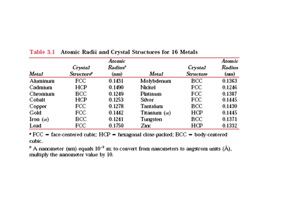
23 Ex: Cr (CCC) A = 52.00 g/mol R = 0.125 nm n = 2  teórica a = 4R/ 3 = 0.2887 nm  actual a R  = a 3 52.002 átomos Cel unit mol g Cel unit volume átomos mol 6.023 x 10 23 Densidade Teórica,  = 7.18 g/cm 3 = 7.19 g/cm 3

24 ALOTROPIA É a característica de um elemento poder existir em mais de uma estrutura cristalina dependendo da temperatura e da pressão. 911 o C, Fe é CCC913 o C, Fe é CFC

25 Ferro To study how iron behaves at elevated temperatures, we would like to design an instrument that can detect (with a 1% accuracy) the change in volume of a 1-cm 3 iron cube when the iron is heated through its polymorphic transformation temperature. At 911 o C, iron is BCC, with a lattice parameter of 0.2863 nm. At 913 o C, iron is FCC, with a lattice parameter of 0.3591 nm. Determine the accuracy required of the measuring instrument. Example 3.6 SOLUTION The volume of a unit cell of BCC iron before transforming is: V BCC = = (0.2863 nm) 3 = 0.023467 nm 3

26 Example 3.6 SOLUTION (Continued) The volume of the unit cell in FCC iron is: V FCC = = (0.3591 nm) 3 = 0.046307 nm 3 But this is the volume occupied by four iron atoms, as there are four atoms per FCC unit cell. Therefore, we must compare two BCC cells (with a volume of 2(0.023467) = 0.046934 nm 3 ) with each FCC cell. The percent volume change during transformation is: The 1-cm 3 cube of iron contracts to 1 - 0.0134 = 0.9866 cm 3 after transforming; therefore, to assure 1% accuracy, the instrument must detect a change of: ΔV = (0.01)(0.0134) = 0.000134 cm 3

27 Índices de Miller Miller indices – Notação curta para descrever algumas direções e planos nos cristais. São escritos entre [ ] e os números negativos são representados por uma barra sobre eles.

28 Coordenadas de alguns pontos na célula unitária, o número refere-se a distância desde a origem em função dos parâmetros do arranjo

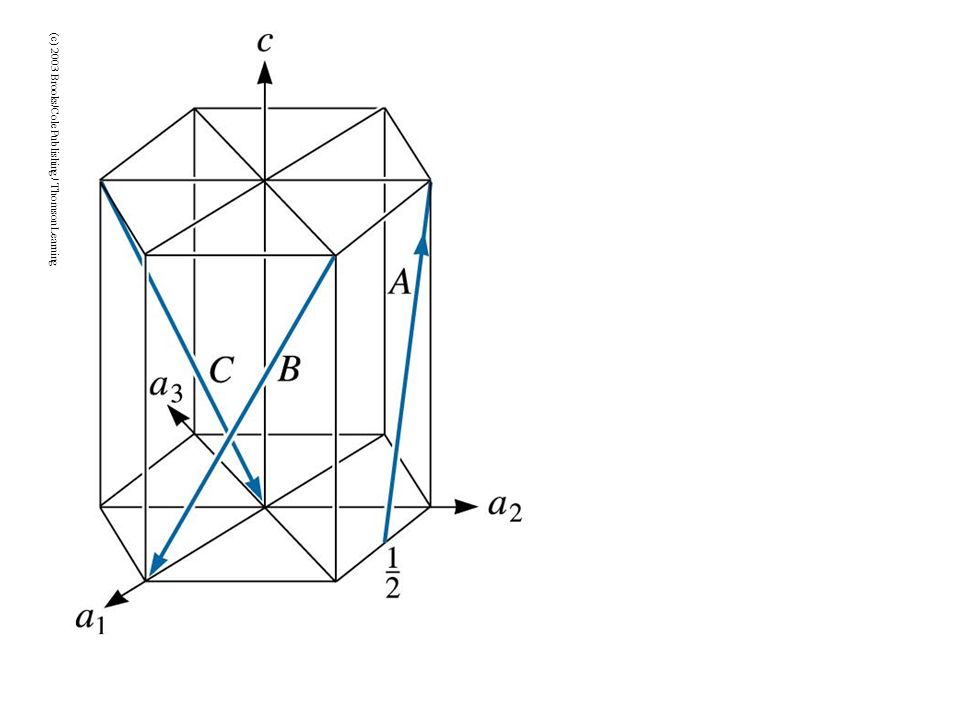
29 Determine os índices de Miller das direções A, B, e C. Determinando os índices de Miller para Direções (c) 2003 Brooks/Cole Publishing / Thomson Learning™

30 Solução Direção A 1. Dois pontos são 1, 0, 0, and 0, 0, 0 2. 1, 0, 0, -0, 0, 0 = 1, 0, 0 3. [100] Direção B 1. Dois pontos são 1, 1, 1 and 0, 0, 0 2. 1, 1, 1, -0, 0, 0 = 1, 1, 1 3. [111] Direção C 1. Dois pontos são 0, 0, 1 and 1/2, 1, 0 2. 0, 0, 1 -1/2, 1, 0 = -1/2, -1, 1 Reduzindo as frações 3. 2(-1/2, -1, 1) = -1, -2, 2 (c) 2003 Brooks/Cole Publishing / Thomson Learning™

31 Determine os índices de Miller dos planos A, B, e C Determinando Índices de Miller de Planos

32 Example 3.8 SOLUTION Plano A 1. x = 1, y = 1, z = 1 2.1/x = 1, 1/y = 1,1 /z = 1 3. Sem frações 4. (111) Plane B 1. O plano nunca cruza o eixo z, x = 1, y = 2, e z = 2.1/x = 1, 1/y =1/2, 1/z = 0 3. Fraçoes: 1/x = 2, 1/y = 1, 1/z = 0 4. (210) Plane C 1. We must move the origin, since the plane passes through 0, 0, 0. Let’s move the origin one lattice parameter in the y- direction. Then, x =, y = -1, and z = 2.1/x = 0, 1/y = 1, 1/z = 0 3. Sem frações.

33 Desenhando direções e planos Draw (a) the direction and (b) the plane in a cubic unit cell.

34 Densidade Linear e Densidade Planar

35 Calculate the planar density and planar packing fraction for the (010) and (020) planes in simple cubic polonium, which has a lattice parameter of 0.334 nm. Calculating the Planar Density and Packing Fraction (c) 2003 Brooks/Cole Publishing / Thomson Learning™ Figure 3.23 The planer densities of the (010) and (020) planes in SC unit cells are not identical (for Example 3.9).

36 Example 3.9 SOLUTION The total atoms on each face is one. The planar density is: The planar packing fraction is given by: However, no atoms are centered on the (020) planes. Therefore, the planar density and the planar packing fraction are both zero. The (010) and (020) planes are not equivalent!

37 We wish to produce a radiation-absorbing wall composed of 10,000 lead balls, each 3 cm in diameter, in a face- centered cubic arrangement. We decide that improved absorption will occur if we fill interstitial sites between the 3-cm balls with smaller balls. Design the size of the smaller lead balls and determine how many are needed. Design of a Radiation-Absorbing Wall (c) 2003 Brooks/Cole Publishing / Thomson Learning™ Figure 3.30 Calculation of an octahedral interstitial site (for Example 3.13).

38 Example 3.13 SOLUTION First, we can calculate the diameter of the octahedral sites located between the 3-cm diameter balls. Figure 3.30 shows the arrangement of the balls on a plane containing an octahedral site. Length AB = 2R + 2r = 2R r = R – R = ( - 1)R r/R = 0.414 This is consistent with Table 3-6. Since r = R = 0.414, the radius of the small lead balls is r = 0.414 * R = (0.414)(3 cm/2) = 0.621 cm. From Example 3-12, we find that there are four octahedral sites in the FCC arrangement, which also has four lattice points. Therefore, we need the same number of small lead balls as large lead balls, or 10,000 small balls.

39 Determining the Density of BCC Iron Determine the density of BCC iron, which has a lattice parameter of 0.2866 nm. Example 3.4 SOLUTION Atoms/cell = 2, a 0 = 0.2866 nm = 2.866  10 -8 cm Atomic mass = 55.847 g/mol Volume of unit cell = = (2.866  10 -8 cm) 3 = 23.54  10 -24 cm 3 /cell Avogadro’s number N A = 6.02  10 23 atoms/mol

40 Determine the packing factor for diamond cubic silicon. Example 3.17 Determining the Packing Factor for Diamond Cubic Silicon (c) 2003 Brooks/Cole Publishing / Thomson Learning Figure 3.39 Determining the relationship between lattice parameter and atomic radius in a diamond cubic cell (for Example 3.17).

41 Example 3.17 SOLUTION We find that atoms touch along the body diagonal of the cell (Figure 3.39). Although atoms are not present at all locations along the body diagonal, there are voids that have the same diameter as atoms. Consequently: Compared to close packed structures this is a relatively open structure.

42 Example 3.18 Calculating the Radius, Density, and Atomic Mass of Silicon The lattice constant of Si is 5.43 Å. What will be the radius of a silicon atom? Calculate the theoretical density of silicon. The atomic mass of Si is 28.1 gm/mol. Example 3.18 SOLUTION For the diamond cubic structure, Therefore, substituting a = 5.43 Å, the radius of silicon atom = 1.176 Å. There are eight Si atoms per unit cell.

43 (c) 2003 Brooks/Cole Publishing / Thomson Learning Figure 3.48 Directions in a cubic unit cell for Problem 3.51

44 (c) 2003 Brooks/Cole Publishing / Thomson Learning Figure 3.49 Directions in a cubic unit cell for Problem 3.52.

45 (c) 2003 Brooks/Cole Publishing / Thomson Learning Figure 3.50 Planes in a cubic unit cell for Problem 3.53.

46 (c) 2003 Brooks/Cole Publishing / Thomson Learning Figure 3.51 Planes in a cubic unit cell for Problem 3.54.

47

48

49

50 Exemplo:

51

52

53 Figure 3.52 Directions in a hexagonal lattice for Problem 3.55. Estrutura Hexagonal com a sua respetiva célula unitária

54 Planos e Direções Cristalográficas Miller–Bravais

55 Planos e Direções Cristalográficas

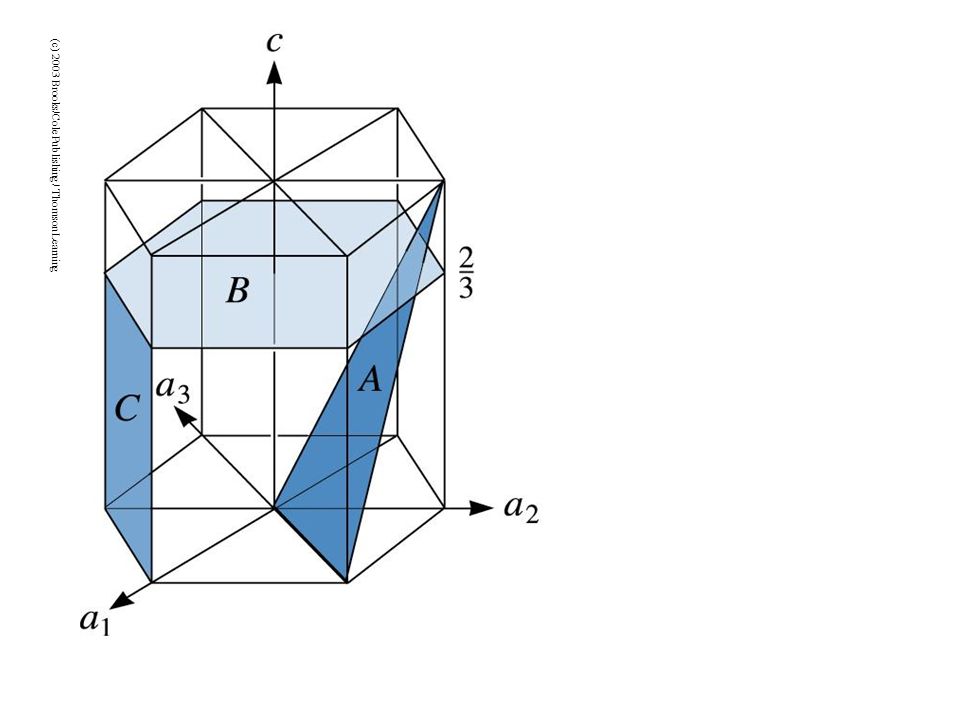
56 Determine the Miller-Bravais indices for planes A and B and directions C and D in Figure 3.25. Determining the Miller-Bravais Indices for Planes and Directions (c) 2003 Brooks/Cole Publishing / Thomson Learning™

57 Example 3.11 SOLUTION Plane A 1. a 1 = a 2 = a 3 =, c = 1 2. 1/a 1 = 1/a 2 = 1/a 3 = 0, 1/c = 1 3. No fractions to clear 4. (0001) Plane B 1. a 1 = 1, a 2 = 1, a 3 = -1/2, c = 1 2. 1/a 1 = 1, 1/a 2 = 1, 1/a 3 = -2, 1/c = 1 3. No fractions to clear 4. Direction C 1. Two points are 0, 0, 1 and 1, 0, 0. 2. 0, 0, 1, -1, 0, 0 = 1, 0, 1 3. No fractions to clear or integers to reduce. 4.

58 Example 3.11 SOLUTION (Continued) Direction D 1. Two points are 0, 1, 0 and 1, 0, 0. 2. 0, 1, 0, -1, 0, 0 = -1, 1, 0 3. No fractions to clear or integers to reduce. 4.

59 (c) 2003 Brooks/Cole Publishing / Thomson Learning

60

61

62 Figure 3.55 Planes in a hexagonal lattice for Problem 3.58.