Da escala micro para a escala nano As técnicas de crescimento epitaxial permitiram a miniaturização Como são produzidos os semicondutores ? MBE – Molecular.

Apresentação em tema: "Da escala micro para a escala nano As técnicas de crescimento epitaxial permitiram a miniaturização Como são produzidos os semicondutores ? MBE – Molecular."— Transcrição da apresentação:

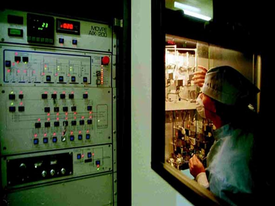
1 Da escala micro para a escala nano As técnicas de crescimento epitaxial permitiram a miniaturização Como são produzidos os semicondutores ? MBE – Molecular Beam Epitaxy CBE – Chemical Beam Epitaxy MOVPE – Metalorganic Vapor Phase Epitaxy

2 MBE Alto vácuo Pressão 10 -10 Torr

3 MOVPE MOCVD - Metalorganic Chemical Vapor Deposition OMCVD - Organometallic Chemical Vapor Deposition OMVPE - Organometallic Vapor Phase Epitaxy

4

5 Princípio de deposição (CH 3 ) 3 Ga + AsH 3 → GaAs + 3 CH 4 (1-x) (CH 3 ) 3 Ga + x(CH 3 ) 3 Al + AsH 3 → Al x Ga 1-x As + 3 CH 4

6

7 TMGa AsH 3 Epitaxial Growth GaAs Substrate

8 GaAs AlAs InP InAs In x Ga 1-x As Ga x Al 1-x As GaP In x Ga 1-x P In x Al 1-x As

9 aa Lattice matched Strained layers GaAs AlGaAs GaAs a’ > a InAs Strained InAs

10 3D a 0D

11 De 3D a 0D 3D E = E g + h 2 k 2 /8m Density of states (E) = 2 1/2 8m c 3/2 (E- E g ) 1/2 /h 3 2D E = Eg + Eq z + h 2 k // 2 /8 2 m Eq z = q z 2 h 2 /8md 2 Density of states (E) = 4m/h 2 1D E = E g +Eq z +Eq y + h 2 k x 2 /8 2 m Eq z,y = q z,y 2 h 2 /8md 2 Density of states (E) = 8Lm 1/2 /h2 ½ (E-E q ) 1/2 0D E = Eg+Eq z +Eq y +Eq x Eq (z,y.x) = q z,y,x 2 h 2 /8md 2 Density of states (E) = # of dots g /Vol

12 Pontos quânticos Estruturas com confinamento 3D numa escala menor que o raio de Bohr levando a uma quantização 3D. Comportamento atômico. 1980 foram fabricados os primeiros pontos quânticos de ZnS em vidro. Existem várias maneiras de produzí-los. O que são estas estruturas 0D?

13 Estrutura de banda

14 Sintonia de estruturas de PQs Fafard 2003

15 Top-down vs bottom-up Top-down: Photolithography Electron beam lithography X-rays Extreme ultraviolet light Scanning probe methods Bottom-up: Self-assembled quantum dots Scanning probe methods

16 Comparando os métodos Lithography Advantage: The electronics industry is already familiar with this technology. Disadvantage: The necessary modifications will be expensive. UV- light and x-rays can damage the equipment. Scanning Probe Advantage: STM and AFM are very versatile, they can move particles in a patterned fashion. Disadvantage: Too slow for mass production. Bottom-up Methods Advantage: Controlled chemical reactions can cheaply and “easily” produce nanostructures. Disadvantage: Cannot produce designed, interconnected patterns.

17 Pontos quânticos auto-organizados

18 Métodos diferentes de crescimento

19 Stranski-Krastanow

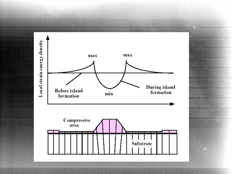
20 Princípio de formação de pontos quânticos por MOVPE Uma diferença importante no parâmetro de rede numa heteroestrutura, leva a um aumento na energia elástica que será aliviada com a formação de ilhas de dimensões que podem ser inferiores ao raio de Bohr. Para materiais descasados um aumento na tensão elástica com o aumento na espessura torna a superfície rugosa. O crescimento 2D camada a camada é interrompido e num segundo passo, a nucleação 3D se inicia. Numa terceira etapa as ilhas 3D se desenvolvem em tamanho consumindo o material que está móvel na superfície. Seifert 2000

21

22 Espessura da wetting layer

23 Dots’ parameters Dot density 10 8 to 10 11 cm 2 Dot size 4 – 20 nm height, 20 – 50 nm base width Dot shape Pyramidal, truncated pyramidal, lens- and cone-shaped How to determine these parameters?

24 Scanning Tunneling Microscopy (Nobel Prize to Rohrer and Binnig in 1986)

25 Atomic Force Microscopy Determination of size distribution and density of quantum dots

26 Example of AFM Results

27 Transmission Electron Microscopy Two geometries: Plain view Cross section Cross section gives information about shape, size and composition. Samples are thinned down to a thickness of the order of 1m. InAs/GaAs 10 4 – 10 6 atoms per dot

28 TEM image of an InAs/InGaAs/InP dot Landi et al 2005 HREM images

29 Photoluminescence The laser beam usually probes an ensemble of quantum dots. The FWHM gives information on the uniformity of the dot size distribution. For a density of 10 10 cm -2, one probes about 10 6 dots for a 100 m laser spot. Single dot spectroscopy requires low dot density and processing to isolate one dot.

30 s p d f Luminescence of an ensemble of dots with resolved excited states. Linewidths of the order of 20-30 meV. Fafard et al 2000 Single dot spectroscopy. Linewidths of the order of eV. Signal is time averaged. Examples of Photoluminescence of Dots Finley et al 2001

31 Electroluminescence for two injection levels reveals the Pauli principle. Photocurrent measurements show absorption to the ground state (s) and to three excited states (p, d, f). Mowbray et al 2005

32 Growth parameters Temperature Higher temperature, lower density, larger size. Deposition time Longer times, more material, larger dots. Fluxes of gases/ Growth rate Higher growth rates, smaller dots, higher density. Annealing time For the same amount of material the dot density and the dot size show inverse behavior

33 T growth = 500°C T growth = 520°C Height increases FWHM decreases Effect of temperature on InAs/InGaAs/InP

34 Reduction of the PL FWHM in agreement with AFM results PL intensity for higher energies decreases → larger dots Effect of temperature on InAs/InGaAs/InP

35 Deposition time increases → Dot density increases InAs/InGaAs/InP

36 In flux: 30 sccm60 sccm66 sccm 76 sccm T growth : 520 o C t growth : 4.2 s InAs / InP In flux / growth rate dependence

37 InAs / InGaAs / InP Attempting to reach higher densities InAs /InP

38 Same scale: from 2.0 10 8 to 2.0 10 10 dots cm -2 InAs/InP T g = 490 o C H  12 nm InAs/InGaAs T g =490 o C H  9 nm

39 Stacks of quantum dots For device applications it is important to have several layers of dots. Nature has helped. In general dots spontaneously grow on top of each other.

40 200 nm Surface QDs Multi-layers of quantum dots 20 nm AFM image TEM Images of Stacked Quantum Dots Landi et al 2005

41 Red-shift with increasing number of stacks Vertical coupling increases the average dot height Effect of number of stacks on dots’ properties Landi et al 2004

42 Controlled site deposition of quantum dots on a patterned surface Patterned substrate using AFM Dots’ formation on designated sites Dots grown away from the patterned region Fonseca Filho et al 2005